Demo: Why the Bell Curve Is Everywhere

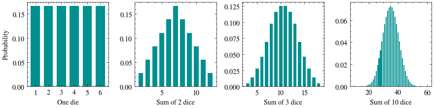
Roll one die and every face is equally likely, so the distribution is flat. Roll ten dice and add them up.

What shape does the distribution of the sum make, and where does it peak? Sketch your guess before we run anything.

import numpy as np
import matplotlib.pyplot as plt
import scienceplots

plt.style.use(["science", "no-latex"])
TEAL = "#009090"

die = np.ones(6) / 6  # a fair die: each face has probability 1/6

fig, axes = plt.subplots(1, 4, figsize=(9, 2.4))
pmf = die.copy()
for ax, k in zip(axes, [1, 2, 3, 10]):
    while len(pmf) < 6 * k - k + 1:      # convolve until pmf is the sum of k dice
        pmf = np.convolve(pmf, die)
    ax.bar(np.arange(k, 6 * k + 1), pmf, color=TEAL, width=0.7)
    ax.set_xlabel(f"Sum of {k} dice" if k > 1 else "One die")
axes[0].set_xticks(np.arange(1, 7))
axes[0].set_ylabel("Probability")
fig.tight_layout()
plt.show()

As we add dice, the distribution changes from flat to triangular and then approaches a bell. From lecture, the expectation of one die is \(\mathbb{E}[X] = 3.5\) and its variance is \(\mathrm{Var}(X) = \frac{35}{12}\). By linearity of expectation, the sum of \(k\) dice has expectation \(3.5k\). Because the dice are independent, every covariance term in the variance of a sum drops out, so the sum has variance \(\frac{35}{12}k\).

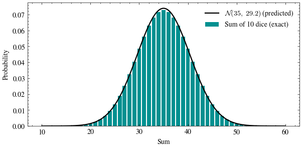
The Gaussian prediction for the sum of ten dice is \(\mathcal{N}(35,\ 350/12)\), determined by the expectation and variance from lecture.

k = 10
pmf = die.copy()
for _ in range(k - 1):
    pmf = np.convolve(pmf, die)
values = np.arange(k, 6 * k + 1)

mu, var = 3.5 * k, (35 / 12) * k
x = np.linspace(values[0], values[-1], 500)
bell = np.exp(-((x - mu) ** 2) / (2 * var)) / np.sqrt(2 * np.pi * var)

fig, ax = plt.subplots(figsize=(7, 3.2))
ax.bar(values, pmf, color=TEAL, width=0.8, label="Sum of 10 dice (exact)")
ax.plot(x, bell, color="black", linewidth=1.6, label=f"$\\mathcal{{N}}({mu:.0f},\\ {var:.1f})$ (predicted)")
ax.set_xlabel("Sum")
ax.set_ylabel("Probability")
ax.legend(frameon=False)
plt.show()

Loading the die

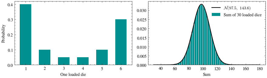
Maybe the bell only appears because the die was fair? Below is a heavily loaded die. Compute the loaded die’s expectation and variance, multiply each by \(k\), and use them to predict the bell.

Change the probabilities to anything you like (they just need to sum to 1). Can you design a die that escapes the bell?

loaded = np.array([0.40, 0.10, 0.05, 0.05, 0.10, 0.30])  # try your own!
faces = np.arange(1, 7)

mu1 = (faces * loaded).sum()               # E[X]
var1 = ((faces - mu1) ** 2 * loaded).sum() # Var(X)

k = 30
pmf = loaded.copy()
for _ in range(k - 1):
    pmf = np.convolve(pmf, loaded)
values = np.arange(k, 6 * k + 1)

mu, var = k * mu1, k * var1
x = np.linspace(values[0], values[-1], 500)
bell = np.exp(-((x - mu) ** 2) / (2 * var)) / np.sqrt(2 * np.pi * var)

fig, (ax1, ax2) = plt.subplots(1, 2, figsize=(9, 2.8))
ax1.bar(faces, loaded, color=TEAL, width=0.6)
ax1.set_xlabel("One loaded die")
ax1.set_ylabel("Probability")
ax2.bar(values, pmf, color=TEAL, width=0.8, label=f"Sum of {k} loaded dice")
ax2.plot(x, bell, color="black", linewidth=1.6, label=f"$\\mathcal{{N}}({mu:.1f},\\ {var:.1f})$")
ax2.set_xlabel("Sum")
ax2.legend(frameon=False, loc="upper right")
fig.tight_layout()
plt.show()

For independent copies of a die, the standardized sum approaches a Gaussian distribution (the central limit theorem). The expectation and variance determine the center and width of the unstandardized sum.

Measurement noise is exactly such a sum of many small independent effects. That is why, when we derive the mean squared error loss in the Linear Models unit, our noise model will be the Gaussian.