Probability
Welcome to the course. By the end of the semester, you will be able to take apart the machinery behind modern deep learning: how a model represents data, how it turns mistakes into a loss, how an optimizer changes millions of parameters, and how we tell whether the result will work on data it has never seen. We will build that understanding from a small set of foundational tools rather than treating each new model as a new trick.
Those tools recur on purpose. Probability gives us estimators, noise models, and generalization; linear algebra gives us linear models, neural-network layers, convolutions, and attention; the singular value decomposition returns in least squares, compression, embeddings, finetuning, and optimization. Near the end of the course, reinforcement learning will bring us back to the Monte Carlo estimators and variance reduction we learn in the opening weeks. The course is cumulative, but in a useful way: each return gives an old idea a new job.
A normal class uses the reading to introduce the mathematics before class, the demo to make one part visible in code, and the problem set for practice. Short quizzes check that those tools are becoming yours; the exams ask you to connect them; and the project gives you room to implement one method on data you care about and explain what you found.
When I tell people I work on machine learning, they want to talk about neural networks and chatbots. Nobody has ever asked me about probability. But almost every question we ask this semester is about random quantities: how well a model will do on unseen data, why one loss is better than another, and why training on small random batches works at all. Today has one goal: build the language that lets us answer those questions, all organized around one puzzle:
Expectation will tell us where a sum of random quantities lands, variance how far it strays, and covariance exactly when that predictability breaks down. Bayes’ rule, at the end, runs the question backwards, from observed evidence to belief about the cause. We begin with events.
Events
Let \(A\) and \(B\) be two events. For example, \(A\) could be the event that it rains tomorrow, and \(B\) the event that I carry an umbrella. We will use the following notation:
- \(\Pr(A)\) is the probability that event \(A\) occurs,
- \(\Pr(A \cup B)\) is the probability that either event occurs,
- \(\Pr(A \cap B)\) is the probability that both events occur,
- \(\Pr(A | B)\) is the probability that event \(A\) occurs given that event \(B\) has occurred.
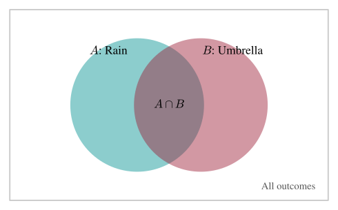
In the plot, each event is the set of outcomes where it happens, and conditioning on \(B\) means we zoom in: \(\Pr(A|B)\) asks what fraction of the circle \(B\) is covered by the overlap \(A \cap B\), where it rains and I carry an umbrella.
We can reason through several properties of probabilities:
Probability Range The probability of an event is always between 0 and 1, i.e., \(0 \leq \Pr(A) \leq 1\) for all events \(A\).
Complement Rule The complement of an event \(A\) is the event that \(A\) does not occur, denoted \(\neg A\). Since exactly one of \(A\) and \(\neg A\) occurs, their probabilities add to one: \[\Pr(\neg A) = 1 - \Pr(A).\]
Union of Events The probability that either event occurs adds the two probabilities and removes the double count: \[\Pr(A \cup B) = \Pr(A) + \Pr(B) - \Pr(A \cap B).\]
Conditional Probabilities We can write the probability of both events occurring in terms of conditional probabilities: \[\Pr(A \cap B) = \Pr(B) \Pr(A | B) = \Pr(A) \Pr(B | A).\] In words: for both events to occur, first one must occur, and then the other must occur given the first.
Independence Two events \(A\) and \(B\) are independent if the occurrence of one does not affect the probability of the other: \[\Pr(A | B) = \Pr(A) \qquad \text{and} \qquad \Pr(B | A) = \Pr(B).\] Combined with the previous property, this gives the form we will use most often: \[\Pr(A \cap B) = \Pr(A) \Pr(B).\] Do you see how the second display follows from the first?
Independence is a strong assumption, and several of the surprises in this course come from assuming it where it does not hold: rain and umbrellas are certainly not independent. Events are all-or-nothing, though, and most of what we want to reason about has a size: how much it rained, how large the loss was. For that, we need numbers.
Random Variables
We will often model random events with random variables, functions that map outcomes to real numbers. For example, let \(X\) be the number showing after we roll a fair six-sided die (the loaded ones we leave to the casinos). The distribution of a random variable describes the probability of each possible value. For our die, \(\Pr(X = x) = \frac16\) for each \(x \in \{1, 2, \ldots, 6\}\).
Distributions do not have to be flat like the die’s. Let \(X_1\) and \(X_2\) be two independent die rolls, and consider their sum \(X_1 + X_2\). There is only one way to roll a 2 but six ways to roll a 7, so the sum piles up in the middle. This is the first hint of our question: one die is anybody’s guess, and already the sum of two is not.
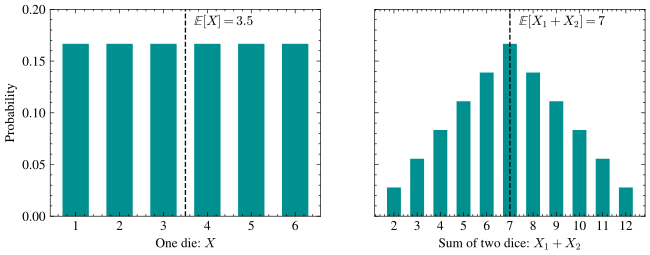
In the plot, the single die is flat and the sum of two is triangular; the dashed lines mark the expectations, which we define next.
Random variables can also be continuous, taking any real value; then the distribution assigns probabilities to ranges of values via a density function. The most important continuous distribution in this course is the Gaussian (or normal) distribution \(\mathcal{N}(\mu, \sigma^2)\), whose density at a point \(x\) is set by two numbers, a center \(\mu\) and a width \(\sigma > 0\): \[ \frac{1}{\sqrt{2\pi \sigma^2}} \exp\left(-\frac{(x - \mu)^2}{2\sigma^2}\right). \]
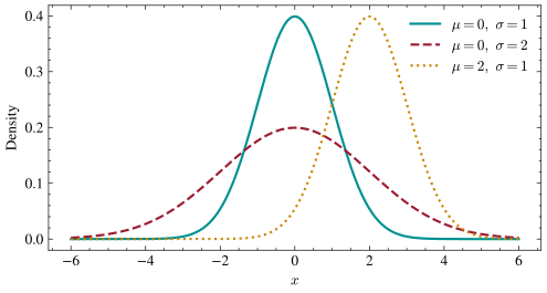
In the plot, increasing \(\sigma\) flattens and widens the bell, changing \(\mu\) slides it without changing its shape, and the exponential decays fast enough that values several \(\sigma\) from the center are very unlikely. The Gaussian appears so often because of a phenomenon the dice previewed: when many independent effects add up, their sum tends toward a bell shape (the central limit theorem). (The class demo pushes this further, stacking up more and more dice until even a loaded one can’t escape the bell.) Measurement noise is often the sum of many small independent effects, which is why we will model noise as Gaussian when we derive the mean squared error loss in the Linear Models unit.
Expectation and variance determine where that limiting bell sits and how wide it is.
Expectation
The expectation of a random variable is the average of its values, weighted by their probabilities: \[ \mathbb{E}[X] = \sum_x x \Pr(X = x), \] where the sum ranges over the values \(X\) can take (for continuous random variables, an integral against the density). Every face of our die is equally likely, so its expectation is the plain average of the six faces: \[ \mathbb{E}[X] = \frac{1 + 2 + 3 + 4 + 5 + 6}{6} = 3.5. \] Notice that the expectation is not a value the die can actually show; it is where the distribution balances.
The most useful property of expectation is linearity of expectation, which holds for any random variables \(X\) and \(Y\) and any constants \(a\) and \(b\): \[ \mathbb{E}[aX + bY] = a\,\mathbb{E}[X] + b\,\mathbb{E}[Y]. \] Linearity does not require independence: \(X\) and \(Y\) may be dependent (\(Y\) could even be \(-X\)). For the sum of two dice, linearity immediately gives \(\mathbb{E}[X_1 + X_2] = 3.5 + 3.5 = 7\), with no need to enumerate the 36 outcomes. Next lecture, linearity proves that our first estimator is correct on average, and the same property returns throughout the course.
Dependence affects the width of a sum, which requires variance and covariance.
Variance and Covariance
Expectation tells us where a distribution centers, but not how much it spreads. The variance measures that spread as the expected squared distance from the mean: \[ \textnormal{Var}(X) = \mathbb{E}\left[(X - \mathbb{E}[X])^2\right]. \] Squaring counts deviations above and below the mean the same, and it penalizes one large deviation far more than several small ones, so the variance is driven by the tails.
Expanding that square gives an equivalent form that is usually easier to compute: \[ \begin{align*} \textnormal{Var}(X) &= \mathbb{E}\left[(X - \mathbb{E}[X])^2\right] \\&= \mathbb{E}\left[X^2 - 2 X\,\mathbb{E}[X] + (\mathbb{E}[X])^2\right] \\&= \mathbb{E}[X^2] - 2\,\mathbb{E}[X]\,\mathbb{E}[X] + (\mathbb{E}[X])^2 \\&= \mathbb{E}[X^2] - (\mathbb{E}[X])^2, \end{align*} \] where we foiled the square, applied linearity of expectation, and used that \(\mathbb{E}[X]\) is a number rather than a random variable, so it slides out of expectations. For our die, \(\mathbb{E}[X^2] = \frac{1 + 4 + 9 + 16 + 25 + 36}{6} = \frac{91}{6}\), so the variance is \(\frac{91}{6} - (3.5)^2 = \frac{35}{12} \approx 2.92\). Its square root is the standard deviation \(\sigma\), which has the same units as \(X\) itself and is exactly the \(\sigma\) in \(\mathcal{N}(\mu, \sigma^2)\).
Shifting a random variable does not change its spread, and scaling it multiplies the spread by the square of the scale: \[ \textnormal{Var}(X + c) = \textnormal{Var}(X) \qquad \text{and} \qquad \textnormal{Var}(aX) = a^2\,\textnormal{Var}(X). \] That square is what makes averaging work: averaging \(n\) samples multiplies their sum by \(\frac1n\), which divides the variance of the sum by \(n^2\) rather than by \(n\), and next lecture the mismatch between those two powers becomes the accuracy of the average.
What about the variance of a sum? Variance is not linear, and the correction term is important enough to get its own name. The covariance measures how two random variables move together: \[ \textnormal{Cov}(X, Y) = \mathbb{E}\left[(X - \mathbb{E}[X])(Y - \mathbb{E}[Y])\right]. \] When \(X\) tends to sit above its mean exactly when \(Y\) does, the product inside is usually positive; think of daily temperature and ice-cream sales, a pair we will meet again when we study regression. When one tends to be high while the other is low, the covariance is negative, and when the two are independent, it is zero (though the converse is false).
Setting \(Y = X\) turns a covariance into a variance. Since expectation is linear, covariance also distributes over sums in each of its two arguments (we say it is bilinear): \[ \textnormal{Cov}(X, X) = \textnormal{Var}(X) \qquad \text{and} \qquad \textnormal{Cov}(X_1 + X_2,\ Y) = \textnormal{Cov}(X_1, Y) + \textnormal{Cov}(X_2, Y). \]
Covariance carries the units of \(X\) times the units of \(Y\), so its raw size tells us little on its own; dividing by the standard deviations \(\sigma_X\) and \(\sigma_Y\) cancels the units and gives the correlation: \[ \rho = \frac{\textnormal{Cov}(X, Y)}{\sigma_X \sigma_Y} \in [-1, 1], \] which reaches \(\pm 1\) exactly when one variable is a linear function of the other and is our dial for how much two random quantities share.
We can now state exactly how variance behaves on sums.
Claim: \(\textnormal{Var}(X + Y) = \textnormal{Var}(X) + \textnormal{Var}(Y) + 2\,\textnormal{Cov}(X, Y)\).
Proof of Claim
Write \(\mu_X = \mathbb{E}[X]\) and \(\mu_Y = \mathbb{E}[Y]\). By linearity of expectation, the mean of the sum is \(\mu_X + \mu_Y\), so the definition of variance gives: \[ \begin{align*} \textnormal{Var}(X + Y) &= \mathbb{E}\left[(X + Y - \mu_X - \mu_Y)^2\right] \\&= \mathbb{E}\left[\left((X - \mu_X) + (Y - \mu_Y)\right)^2\right] \\&= \mathbb{E}\left[(X - \mu_X)^2\right] + \mathbb{E}\left[(Y - \mu_Y)^2\right] + 2\,\mathbb{E}\left[(X - \mu_X)(Y - \mu_Y)\right] \\&= \textnormal{Var}(X) + \textnormal{Var}(Y) + 2\,\textnormal{Cov}(X, Y), \end{align*} \] where we grouped the deviations, foiled the square, and applied linearity of expectation to split the three terms.The cross term is the mechanism: squaring the sum multiplies the two deviations, which reinforce each other when both variables sit above their means at once, so positive covariance widens the sum’s swings, negative covariance narrows them, and when \(X\) and \(Y\) are independent the covariance vanishes and the variances simply add.
The same expansion runs for a sum of \(n\) random variables, where every variance appears once and every pair of variables contributes a covariance. On the problem set, you will carry out that generalization and use it to answer a real puzzle: why a poll of 10,000 people can still miss the true answer by three points. The problem set applies this expansion to a poll with correlated responses.
Bayes’ Rule
Conditional probabilities have a direction, and it is often not the direction we need. A doctor may know from studies how likely a symptom is given a disease, while a patient wants to know how likely the disease is given the symptom. Bayes’ rule reverses the conditioning for any two events \(A\) and \(B\) with \(\Pr(B) > 0\): \[ \Pr(A | B) = \frac{\Pr(B | A) \Pr(A)}{\Pr(B)}. \] Based on the properties of events we saw earlier, can you prove Bayes’ rule? (One of them is enough.)
Each factor has a name that we will use throughout the course. The left-hand side \(\Pr(A|B)\) is the posterior: what we believe about \(A\) after seeing the evidence \(B\). On the right, \(\Pr(B|A)\) is the likelihood of the evidence when \(A\) holds, \(\Pr(A)\) is the prior belief before any evidence, and \(\Pr(B)\) is the total probability of the evidence. The evidence term is often computed by splitting over whether \(A\) occurred: \[ \Pr(B) = \Pr(B|A)\Pr(A) + \Pr(B|\neg A)\Pr(\neg A). \]
A Medical Test
The medical-test example shows why the prior matters in this calculation. Suppose a disease affects 1% of the population. There is a test for it, but the test is imperfect: it has a false positive rate of 5% (healthy patients test positive 5% of the time) and a false negative rate of 10% (sick patients test negative 10% of the time). You take the test.
Most people answer somewhere around 90%, reasoning that the test is right almost all of the time. The computation is the class exercise, and it lands somewhere else entirely: a positive result from this 90%-accurate test leaves you with only a 15% chance of having the disease.
Solution to the class exercise
Let \(D\) be the event that you have the disease and \(+\) the event that the test is positive. The problem gives us the prior \(\Pr(D) = 0.01\), the false positive rate \(\Pr(+ | \neg D) = 0.05\), and, via the complement rule, the likelihood \(\Pr(+ | D) = 1 - 0.10 = 0.90\). Bayes’ rule assembles those three numbers into the posterior, with the evidence term split over whether you are sick: \[ \Pr(D | +) = \frac{\Pr(+ | D) \Pr(D)}{\Pr(+ | D)\Pr(D) + \Pr(+ | \neg D)\Pr(\neg D)} = \frac{0.90 \cdot 0.01}{0.90 \cdot 0.01 + 0.05 \cdot 0.99} = \frac{0.009}{0.0585} \approx 0.15. \]If that answer feels wrong, counting a concrete population usually makes it feel right. Imagine 10,000 people taking the test: on average 100 of them are sick and 90 of those test positive, while of the 9,900 healthy people 5% (about 495) also test positive. So 585 people walk away with a positive result, and only \(\frac{90}{585} \approx 15\%\) of them are sick.
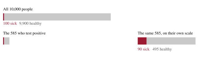
In the plot, the positive test barely thins the sick while eliminating most of the healthy; the right panel puts the 585 positives on their own scale, where the 90 sick are the dark red block at the left end. The disease is rare enough that the mostly-healthy crowd produces more false positives than there are sick people in the entire population. The test is still informative, since it multiplied our belief from 1% to 15%, but a strong prior takes strong evidence to overturn.
This pattern of updating a prior with evidence returns all semester: when we derive logistic regression in the Linear Models unit, the sigmoid function will fall out of exactly this posterior calculation, and when we study generalization, priors will reappear as regularization.
Monte Carlo Estimation
Next lecture, we meet our first algorithm: the Monte Carlo estimator, which approximates an unknown quantity by averaging independent random samples. Expectation gives this estimator’s mean, while variance and covariance quantify its error. Variance reduction returns in stochastic gradient descent and reinforcement learning. For sums of random quantities, independence determines whether averaging reduces the variance at the usual rate.