Demo: To Learn an Average, Take an Average

Roll two dice and keep the larger value: rolling with advantage. Its long-run average is \(\mu = \mathbb{E}[\max(X_1, X_2)]\).

This game is small enough to enumerate, so all \(36\) outcomes give us \(\mu\) and \(\sigma^2\) exactly.

import numpy as np
import matplotlib.pyplot as plt
import scienceplots

plt.style.use(["science", "no-latex"])
TEAL, CARDINAL = "#009090", "#9c1b33"
rng = np.random.default_rng(0)

outcomes = [(i, j) for i in range(1, 7) for j in range(1, 7)]
mu = np.mean([max(i, j) for i, j in outcomes])
sigma2 = np.mean([(max(i, j) - mu) ** 2 for i, j in outcomes])
print(f"exact mean      mu      = {mu:.4f}  (= 161/36)")
print(f"exact variance  sigma^2 = {sigma2:.4f}  (= 2555/1296)")
print(f"one-game spread sigma   = {np.sqrt(sigma2):.4f}")

exact mean      mu      = 4.4722  (= 161/36)
exact variance  sigma^2 = 1.9715  (= 2555/1296)
one-game spread sigma   = 1.4041

Now pretend we can’t enumerate: twenty dice, rerolls, a rulebook of modifiers, or a model’s error on every photo on the internet. We can still play. The Monte Carlo estimator plays \(n\) games and averages them:

\[\hat{\mu}_n = \frac{1}{n}\sum_{i=1}^n f(X^{(i)}), \qquad f(X) = \max(X_1, X_2),\]

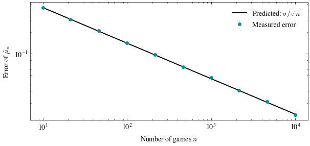
where \(X^{(i)}\) is the \(i\)-th game, a fresh pair of dice. In class we proved this is unbiased, and lecture also predicts its error: \(\sigma/\sqrt{n} \approx 1.40/\sqrt{n}\).

Before running: how many games do we need for one decimal place of accuracy? For two?

ns = np.unique(np.logspace(1, 4, 10).astype(int))
reps = 1000  # replay each experiment many times to measure the typical error

errors = []
for n in ns:
    dice = rng.integers(1, 7, size=(reps, n, 2), dtype=np.int8)
    estimates = dice.max(axis=2).mean(axis=1)
    errors.append(estimates.std())

fig, ax = plt.subplots(figsize=(7, 3))
ax.loglog(ns, np.sqrt(sigma2 / ns), color="black", linewidth=1.4,
          label=r"Predicted: $\sigma/\sqrt{n}$")
ax.loglog(ns, errors, "o", color=TEAL, markersize=4, label="Measured error")
ax.set_xlabel(r"Number of games $n$")
ax.set_ylabel(r"Error of $\hat{\mu}_n$")
ax.legend(frameon=False)
plt.show()

A straight line of slope \(-\frac{1}{2}\) on log-log axes: the \(1/\sqrt{n}\) rate, exactly as predicted. Each extra digit of accuracy costs \(100\times\) more games.

Reducing variance with the same samples

The sum of the two dice is a surrogate with a known mean: \(\mathbb{E}[X_1 + X_2] = 7\) by linearity, with no enumeration at all. When the sum runs high the max probably runs high too, so subtract off the measured luck:

\[\hat{\mu}_c = \frac{1}{n}\sum_{i=1}^n \left[ f(X^{(i)}) - c\,\big(g(X^{(i)}) - 7\big) \right], \qquad g(X) = X_1 + X_2.\]

In class we proved this is unbiased for every \(c\). Guess \(c = \tfrac{1}{2}\), since the max is roughly half the sum.

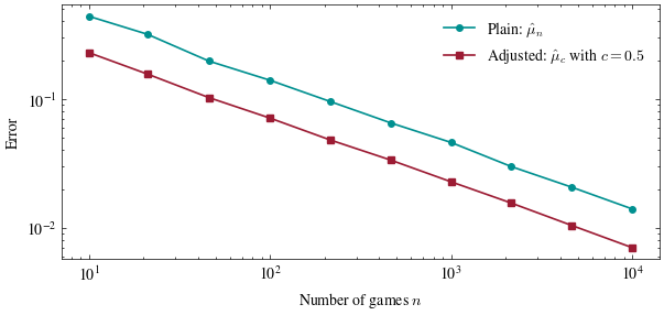
c = 0.5

errors_plain, errors_adj = [], []
for n in ns:
    dice = rng.integers(1, 7, size=(reps, n, 2), dtype=np.int8)
    maxes, sums = dice.max(axis=2), dice.sum(axis=2)
    errors_plain.append(maxes.mean(axis=1).std())
    errors_adj.append((maxes - c * (sums - 7)).mean(axis=1).std())

fig, ax = plt.subplots(figsize=(7, 3))
ax.loglog(ns, errors_plain, "o-", color=TEAL, markersize=4, linewidth=1.2,
          label=r"Plain: $\hat{\mu}_n$")
ax.loglog(ns, errors_adj, "s-", color=CARDINAL, markersize=4, linewidth=1.2,
          label=rf"Adjusted: $\hat{{\mu}}_c$ with $c = {c}$")
ax.set_xlabel(r"Number of games $n$")
ax.set_ylabel("Error")
ax.legend(frameon=False)
plt.show()

Parallel lines, but the adjusted one runs about \(2\times\) lower: the same samples, the accuracy of \(4n\) games. No new rolls were needed, only arithmetic on side information we already had.

Varying the coefficient \(c\)

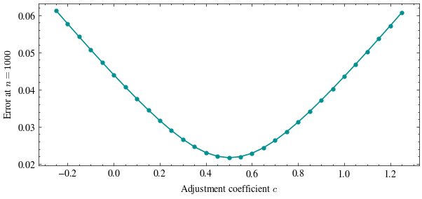
Try values of \(c\) on both sides of \(\tfrac{1}{2}\), including negative and large values.

cs = np.linspace(-0.25, 1.25, 31)
n = 1000

dice = rng.integers(1, 7, size=(reps, n, 2), dtype=np.int8)
maxes, sums = dice.max(axis=2), dice.sum(axis=2)
errors_c = [(maxes - c * (sums - 7)).mean(axis=1).std() for c in cs]

fig, ax = plt.subplots(figsize=(7, 3))
ax.plot(cs, errors_c, "o-", color=TEAL, markersize=3.5, linewidth=1.2)
ax.set_xlabel(r"Adjustment coefficient $c$")
ax.set_ylabel(rf"Error at $n = {n}$")
plt.show()

A quantity correlated with the target and with a known mean can reduce variance without additional samples.

The error traces a curve with a bottom. Problem 2 finds that bottom in closed form and shows that the correlation \(\rho\) between \(f\) and \(g\) sets exactly how much the adjustment can save. Correlation inflated the variance of a sum last week; here it shrinks the estimator’s variance instead.