Demo: Estimating the Larger Die

Roll two fair dice and keep the larger value. We will enumerate the possible outcomes to obtain an exact benchmark, then use simulation to estimate the same quantity.

The demo follows four questions: What are we estimating? Why does averaging more games help? Can information from the same rolls give a better estimate? Which control gives the smallest variance?

import numpy as np
import matplotlib.pyplot as plt

plt.style.use("../figure_style.mplstyle")
rng = np.random.default_rng(0)

Question 1: What Is the Target?

One game produces one score: the larger of the two rolls. This small example has only \(36\) possible pairs, so we can list them and calculate the exact mean and variance. In a larger problem, a simulator would produce the scores instead.

scores = []
for first_die in range(1, 7):
    for second_die in range(1, 7):
        scores.append(max(first_die, second_die))
scores = np.array(scores)

exact_mean = scores.mean()
score_variance = scores.var()
print(f"Exact mean:     {exact_mean:.4f}")
print(f"Score variance: {score_variance:.4f}")

Exact mean:     4.4722
Score variance: 1.9715

Answer. The target is the exact mean, \(\mu \approx 4.47\). The score variance describes how much the result of one game changes from roll to roll. This value gives us a benchmark for the estimator’s variance.

Question 2: Why Average More Games?

Suppose one experiment consists of \(n\) games and reports their average score. To see how that estimate varies, we repeat the entire experiment \(1{,}000\) times. Each die has its own array: rows are repetitions and columns are games. np.maximum keeps the larger die in each game, and mean(axis=1) averages the games in each row.

The final two columns compare the variance across the repeated estimates with the prediction from the reading, \(\operatorname{Var}(f(X))/n\).

n_values = [10, 100, 1000]
repetitions = 1000

print(f"{'Games':>6}  {'Mean estimate':>13}  {'Measured variance':>17}  {'Predicted variance':>18}")
for n in n_values:
    first_die = rng.integers(1, 7, size=(repetitions, n))
    second_die = rng.integers(1, 7, size=(repetitions, n))
    scores = np.maximum(first_die, second_die)
    estimates = scores.mean(axis=1)
    measured_variance = estimates.var(ddof=1)
    predicted_variance = score_variance / n
    print(
        f"{n:6d}  {estimates.mean():13.4f}  "
        f"{measured_variance:17.5f}  {predicted_variance:18.5f}"
    )

 Games  Mean estimate  Measured variance  Predicted variance
    10         4.4794            0.18098             0.19715
   100         4.4733            0.01997             0.01971
  1000         4.4741            0.00209             0.00197

Answer. Every row remains close to \(4.47\), while increasing \(n\) by a factor of ten reduces the variance by about the same factor. The simulation agrees with the \(1/n\) variance formula. More games make the estimate more stable, but they also require more work.

Question 3: Can the Same Rolls Give a Better Estimate?

For each constant \(c\), let \(g_c(X)\) be \(c\) times the sum of the two dice. This control has known mean \(7c\) and moves with the maximum: when the sum is unusually high, the maximum tends to be high. Choosing \(c=0.5\) gives one function in this family. We subtract its centered value, \(g_c(X)-7c\), to correct for some of that shared randomness.

The next cell compares the plain and adjusted estimates using exactly the same simulated games. This isolates the effect of the adjustment.

n = 100
first_die = rng.integers(1, 7, size=(repetitions, n))
second_die = rng.integers(1, 7, size=(repetitions, n))
maximum = np.maximum(first_die, second_die)
total = first_die + second_die

plain_estimates = maximum.mean(axis=1)
c = 0.5
adjusted_scores = maximum - c * (total - 7)
adjusted_estimates = adjusted_scores.mean(axis=1)

print(f"Plain mean:        {plain_estimates.mean():.4f}")
print(f"Plain variance:    {plain_estimates.var(ddof=1):.5f}")
print(f"Adjusted mean:     {adjusted_estimates.mean():.4f}")
print(f"Adjusted variance: {adjusted_estimates.var(ddof=1):.5f}")

Plain mean:        4.4722
Plain variance:    0.02068
Adjusted mean:     4.4683
Adjusted variance: 0.00525

Answer. Both methods remain centered near the same target, but the adjusted estimate has less than one third as much variance. Both estimators use the same rolls. The adjusted estimator reduces error by using the known mean of a related quantity.

Question 4: Which Control Has the Smallest Variance?

The choice \(c=0.5\) was a guess. Each value of \(c\) selects a different function \(g_c\). A value that is too small may leave useful information unused, while one that is too large may overcorrect. We compare several controls on the same rolls. When \(c=0\), \(g_0\) is the zero function, so the adjusted estimator becomes the plain estimator.

c_values = np.array([0.00, 0.25, 0.50, 0.75, 1.00])
sampling_variances = []

for c in c_values:
    adjusted_scores = maximum - c * (total - 7)
    estimates = adjusted_scores.mean(axis=1)
    sampling_variances.append(estimates.var(ddof=1))

fig, ax = plt.subplots(figsize=(7, 3.5))
ax.plot(c_values, sampling_variances, marker="o", linestyle="-", label="Measured Variance")
ax.axvline(0.5, linestyle="--", label="Best Tested Control")
ax.set_xlabel(r"Value of $c$ in $g_c$")
ax.set_ylabel("Variance Across Repeated Estimates")
ax.set_title("Choosing a Control Variate")
ax.legend(frameon=False)
plt.show()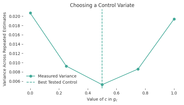

Answer. The variance falls as \(c\) moves from \(0\) to \(0.5\), then rises again. For this game, \(g_{0.5}\) removes the most variance among the controls tested. The problem set derives why \(c=0.5\) gives the best function in this family.

The broader lesson is that a correlated quantity with a known mean can make a Monte Carlo estimate more stable. The estimator still targets the same mean. Only its variance changes.