Demo: A Matrix Moves the Plane

A matrix is a function: it sends every point of the plane somewhere else. Its columns specify where the basis vectors \(\mathbf{e}_1 = (1,0)\) and \(\mathbf{e}_2 = (0,1)\) land.

Before running: the matrix below has columns \((0.87, 0.5)\) and \((-0.5, 0.87)\). What do you think it does to the plane?

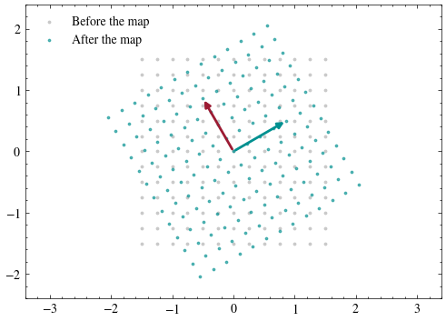
import numpy as np
import matplotlib.pyplot as plt
import matplotlib.cbook as cbook
import scienceplots

plt.style.use(["science", "no-latex"])
TEAL, CARDINAL, GRAY = "#009090", "#9c1b33", "#c9c9c9"

theta = np.pi / 6
A_rot = np.array([[np.cos(theta), -np.sin(theta)],
                  [np.sin(theta),  np.cos(theta)]])

ticks = np.linspace(-1.5, 1.5, 13)
gx, gy = np.meshgrid(ticks, ticks)
points = np.vstack([gx.ravel(), gy.ravel()])   # one point per column


def show_map(A):
    mapped = A @ points
    fig, ax = plt.subplots(figsize=(7, 4.2))
    ax.scatter(points[0], points[1], s=3, color=GRAY, label="Before the map")
    ax.scatter(mapped[0], mapped[1], s=3, color=TEAL, alpha=0.6, label="After the map")
    # the two arrows are the two columns of A: where e1 and e2 land
    ax.annotate("", xy=A[:, 0], xytext=(0, 0),
                arrowprops=dict(arrowstyle="-|>", color=TEAL, linewidth=2))
    ax.annotate("", xy=A[:, 1], xytext=(0, 0),
                arrowprops=dict(arrowstyle="-|>", color=CARDINAL, linewidth=2))
    ax.set_xlim(-3.4, 3.4)
    ax.set_ylim(-2.4, 2.4)
    ax.set_aspect("equal")
    ax.legend(frameon=False, loc="upper left")
    plt.show()


show_map(A_rot)

A rotation by \(30^\circ\), and the two arrows (where \(\mathbf{e}_1\) and \(\mathbf{e}_2\) landed) are exactly the columns of \(\mathbf{A}^{\mathrm{rot}}\).

Next, apply a diagonal matrix.

A_scale = np.array([[2.0, 0.0],
                    [0.0, 0.5]])

show_map(A_scale)

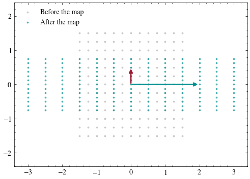
Stretch by \(2\) along \(x\), squash by \(\tfrac12\) along \(y\). Again, read the columns.

Applying the map to a photograph

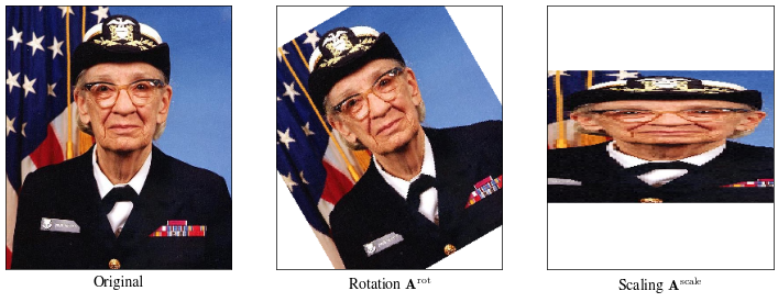
Every pixel has a coordinate, so a \(2 \times 2\) matrix can move a whole photograph. To warp an image we run the map backwards: for each output pixel, ask \(\mathbf{A}^{-1}\) which input pixel it came from.

img = plt.imread(cbook.get_sample_data("grace_hopper.jpg"))[::2, ::2]


def warp(img, A):
    H, W = img.shape[:2]
    ys, xs = np.mgrid[0:H, 0:W]
    xc, yc = xs - W / 2, H / 2 - ys              # pixel indices -> centered xy coordinates
    Ainv = np.linalg.inv(A)
    u = Ainv[0, 0] * xc + Ainv[0, 1] * yc        # where did this output point come from?
    v = Ainv[1, 0] * xc + Ainv[1, 1] * yc
    xi, yi = np.round(u + W / 2).astype(int), np.round(H / 2 - v).astype(int)
    ok = (0 <= xi) & (xi < W) & (0 <= yi) & (yi < H)
    out = np.full_like(img, 255)
    out[ys[ok], xs[ok]] = img[yi[ok], xi[ok]]
    return out


fig, axes = plt.subplots(1, 3, figsize=(9, 3.4))
for ax, M, label in [(axes[0], np.eye(2), "Original"),
                     (axes[1], A_rot, "Rotation $\\mathbf{A}^{\\mathrm{rot}}$"),
                     (axes[2], A_scale, "Scaling $\\mathbf{A}^{\\mathrm{scale}}$")]:
    ax.imshow(warp(img, M))
    ax.set_xlabel(label)
    ax.set_xticks([])
    ax.set_yticks([])
plt.show()

Moving the columns toward parallel

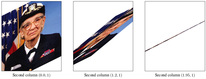
Your turn: edit the matrices below and try your own rotations, stretches, and combinations. All three share the first column \((1, 0.5)\), while the second column slides to the right toward \((2, 1)\), which is exactly twice the first. At \((2, 1)\) the matrix is the reading’s \(\mathbf{A}^{\mathrm{flat}}\), which has no inverse, so we stop just short of it. Watch what happens to the photo as the two columns approach parallel.

fig, axes = plt.subplots(1, 3, figsize=(9, 3.4))
for ax, a in zip(axes, [0.0, 1.2, 1.95]):   # try your own values; a = 2.0 is singular
    M = np.array([[1.0, a],
                  [0.5, 1.0]])
    ax.imshow(warp(img, M))
    ax.set_xlabel(f"Second column $({a}, 1)$")
    ax.set_xticks([])
    ax.set_yticks([])
plt.show()

As the second column closes in on twice the first, the photo is squeezed onto a single line. A rank-\(1\) matrix maps the plane onto one dimension. Only full-rank matrices have inverses because a line cannot be mapped back to the original photograph.

A matrix is a function: its columns are the images of the basis vectors, and its rank is the dimension of its output space. Next lecture studies the directions a matrix stretches without rotating, its eigenvectors.