Demo: The Power Method

Repeated matrix multiplication can reveal a matrix’s leading eigenvector. We will first make the special directions visible, then measure both the method’s convergence and its dependence on the eigengap.

Question 1: Which Directions Are Not Turned?

Consider

\[ \mathbf A=\begin{bmatrix}2&1\\1&2\end{bmatrix}. \]

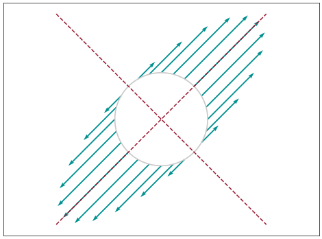
At each point \(\mathbf x\) on the unit circle, the plot draws the change from \(\mathbf x\) to \(\mathbf A\mathbf x\). Look for directions where the arrow stays on the same line.

import numpy as np
import matplotlib.pyplot as plt

plt.style.use("../figure_style.mplstyle")

A = np.array([[2.0, 1.0], [1.0, 2.0]])
v1 = np.array([1.0, 1.0]) / np.sqrt(2)
v2 = np.array([1.0, -1.0]) / np.sqrt(2)

angles = np.linspace(0, 2 * np.pi, 24, endpoint=False)
points = np.array([np.cos(angles), np.sin(angles)])
mapped = A @ points
changes = mapped - points

fig, ax = plt.subplots(figsize=(6, 4.4))
circle = np.linspace(0, 2 * np.pi, 200)
ax.plot(np.cos(circle), np.sin(circle), linewidth=1.2)
ax.quiver(points[0], points[1], changes[0], changes[1],
          angles="xy", scale_units="xy", scale=1, width=0.004)
for v in [v1, v2]:
    ax.plot([-3.2 * v[0], 3.2 * v[0]], [-3.2 * v[1], 3.2 * v[1]],
            linestyle="--", linewidth=1.1)
ax.set_xlim(-3.4, 3.4)
ax.set_ylim(-2.5, 2.5)
ax.set_aspect("equal")
ax.set_xticks([])
ax.set_yticks([])
plt.show()

Answer. Along \(\mathbf v_1=(1,1)/\sqrt2\), the matrix stretches by \(3\). Along \(\mathbf v_2=(1,-1)/\sqrt2\), it leaves vectors unchanged. Other directions contain both components, so the larger factor turns them toward \(\mathbf v_1\).

Question 2: Does Repeated Multiplication Find the Leading Direction?

Starting from \(\mathbf q^{(0)}=(1,0)\), the power method repeatedly multiplies and normalizes:

\[ \mathbf q^{(k)}= \frac{\mathbf A\mathbf q^{(k-1)}} {\lVert\mathbf A\mathbf q^{(k-1)}\rVert_2}. \]

q = np.array([1.0, 0.0])
iterates = [q]
for k in range(10):
    w = A @ q
    q = w / np.linalg.norm(w)
    iterates.append(q)

print(f"target v1      = ({v1[0]:.6f}, {v1[1]:.6f})")
for k in [0, 1, 2, 3, 5, 10]:
    qk = iterates[k]
    print(f"iteration {k:2d}   = ({qk[0]:.6f}, {qk[1]:.6f})")

target v1      = (0.707107, 0.707107)
iteration  0   = (1.000000, 0.000000)
iteration  1   = (0.894427, 0.447214)
iteration  2   = (0.780869, 0.624695)
iteration  3   = (0.732793, 0.680451)
iteration  5   = (0.710011, 0.704191)
iteration 10   = (0.707119, 0.707095)

Answer. The iterates rapidly approach \(\mathbf v_1\). Normalization prevents their length from exploding while preserving the direction created by each multiplication.

Question 3: Can We Predict the Error at Every Step?

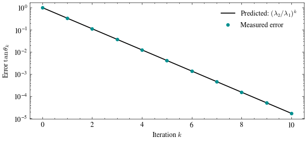
Relative to the leading component, the unwanted \(\mathbf v_2\) component is multiplied by \(\lambda_2/\lambda_1=1/3\) each iteration. We measure that ratio and compare it with the exact prediction \((1/3)^k\).

iterations = np.arange(len(iterates))
errors = []
for q in iterates:
    leading_component = abs(q @ v1)
    other_component = abs(q @ v2)
    errors.append(other_component / leading_component)

fig, ax = plt.subplots(figsize=(7, 3))
ax.semilogy(iterations, (1 / 3.0) ** iterations, linewidth=1.3,
            label=r"Predicted: $(\lambda_2/\lambda_1)^k$")
ax.semilogy(iterations, errors, "o", markersize=4, label="Measured error")
ax.set_xlabel("Iteration $k$")
ax.set_xticks(range(0, 11, 2))
ax.set_ylabel(r"Error $\tan\theta^{(k)}$")
ax.legend(frameon=False)
plt.show()

Answer. The measured points lie on the predicted line. On a log scale, repeated multiplication by a constant becomes a straight line.

Question 4: Why Does the Eigengap Matter?

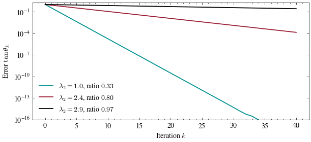
We keep the eigenvectors and \(\lambda_1=3\) fixed, then move \(\lambda_2\) closer to \(\lambda_1\). A ratio near one removes the leading direction’s per-step advantage.

lambda2_values = [1.0, 2.4, 2.9]  # Try other positive values below 3.
linestyles = ["-", "--", ":"]

fig, ax = plt.subplots(figsize=(7, 3))
for lambda2, linestyle in zip(lambda2_values, linestyles):
    comparison_matrix = 3 * np.outer(v1, v1) + lambda2 * np.outer(v2, v2)
    q = np.array([1.0, 0.0])
    errors = [1.0]
    for _ in range(40):
        w = comparison_matrix @ q
        q = w / np.linalg.norm(w)
        leading_component = abs(q @ v1)
        other_component = abs(q @ v2)
        errors.append(other_component / leading_component)
    ax.semilogy(errors, linestyle=linestyle,
                label=rf"$\lambda_2 = {lambda2}$, ratio ${lambda2 / 3:.2f}$")
ax.set_xlabel("Iteration $k$")
ax.set_ylabel(r"Error $\tan\theta^{(k)}$")
ax.set_ylim(1e-16, 2)
ax.legend(frameon=False)
plt.show()

Answer. Convergence slows as \(\lambda_2/\lambda_1\) approaches one. The power method is fast when the leading eigenvalue is clearly separated and slow when competing directions are stretched by nearly the same amount.