Demo: Fitting a Calibration Line

A sensor produces a raw reading \(x\) and we have reference measurements \(y\) from calibration. We will hold these observations fixed while changing the intercept \(b\) and slope \(w\) in \(\widehat y=wx+b\). All measurements are simulated, so the notebook needs no download.

A Candidate Rule

Predict whether the candidate line tends to overpredict or underpredict at each end of the observed range. The vertical segments are the residuals whose squares enter MSE.

import numpy as np
import matplotlib.pyplot as plt

plt.style.use("../figure_style.mplstyle")

The seed keeps the same simulated measurements each time we rerun. Change w or b to compare candidate lines on those fixed observations.

rng = np.random.default_rng(5)
x = np.linspace(-1, 1, 30)
y = 1.5 + 0.8 * x + rng.normal(0, 0.3, len(x))
w = 0.2  # Edit the slope and intercept, then rerun the notebook.
b = 1.0
y_hat = b + w * x

fig, ax = plt.subplots(figsize=(7, 3.5))
ax.scatter(x, y, edgecolors="none", label="Calibration Labels")
ax.plot(x, y_hat, label="Candidate Line")
ax.vlines(x, y_hat, y, linewidth=1)
ax.set_xlabel("x")
ax.set_ylabel("label y")
ax.legend(frameon=False)
plt.show()
print(f"Candidate MSE: {np.mean((y - y_hat) ** 2):.4f}")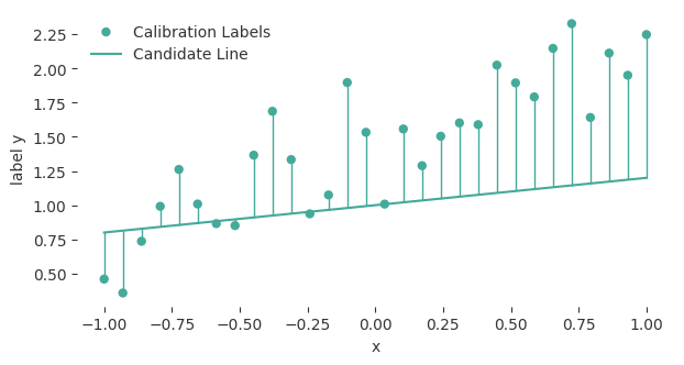

Candidate MSE: 0.3647

The candidate’s residuals are the vertical differences between the line and the observed labels. A larger intercept raises all predictions. A larger slope raises predictions at positive \(x\) and lowers them at negative \(x\).

The Best Line

The reading derives the best slope from centered features and labels, then finds the corresponding intercept. Predict whether the best line must pass through any observed point before calculating it.

centered_x = x - np.mean(x)
centered_y = y - np.mean(y)
w_fit = np.sum(centered_x * centered_y) / np.sum(centered_x ** 2)
b_fit = np.mean(y) - w_fit * np.mean(x)
fit = b_fit + w_fit * x
constant = np.mean(y)

fig, ax = plt.subplots(figsize=(7, 3.5))
ax.scatter(x, y, edgecolors="none", label="Calibration Labels")
ax.plot(x, fit, label="Fitted Line")
ax.axhline(constant, linestyle=":", label="Best Constant")
ax.plot(x, y_hat, linestyle="--", label="Candidate Line")
ax.set_xlabel("x")
ax.set_ylabel("label y")
ax.legend(frameon=False)
plt.show()
print(f"Fitted intercept: {b_fit:.3f}, fitted slope: {w_fit:.3f}")
print(f"Fitted MSE: {np.mean((y - fit) ** 2):.4f}")
print(f"Constant MSE: {np.mean((y - constant) ** 2):.4f}")
assert np.mean((y - fit) ** 2) <= np.mean((y - constant) ** 2) + 1e-12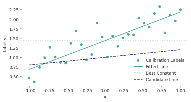

Fitted intercept: 1.435, fitted slope: 0.752
Fitted MSE: 0.0669
Constant MSE: 0.2684

The fit minimizes the combined squared residuals. It need not pass through an observation. The constant predictor is one candidate line with slope zero, so allowing a slope cannot worsen the optimal training MSE.

All Parameter Choices at Once

A contour joins intercept-slope pairs with the same MSE. Predict where the candidate and fitted parameters will appear relative to the smallest contours.

intercepts = np.linspace(0, 3, 100)
slopes = np.linspace(-0.5, 2, 100)
losses = np.zeros((len(slopes), len(intercepts)))
for row, slope in enumerate(slopes):
    for column, intercept in enumerate(intercepts):
        predictions = slope * x + intercept
        losses[row, column] = np.mean((y - predictions) ** 2)

fig, ax = plt.subplots(figsize=(7, 4))
contours = ax.contour(intercepts, slopes, losses, levels=12, cmap="viridis")
fig.colorbar(contours, ax=ax, label="Mean Squared Error")
ax.scatter(b_fit, w_fit, marker="*", s=120, label="Fitted Parameters")
ax.scatter(b, w, marker="x", s=60, label="Candidate Parameters")
ax.set_xlabel("Intercept")
ax.set_ylabel("Slope")
ax.legend(frameon=False, loc="lower center", bbox_to_anchor=(0.5, 1.02), ncol=2)
plt.show()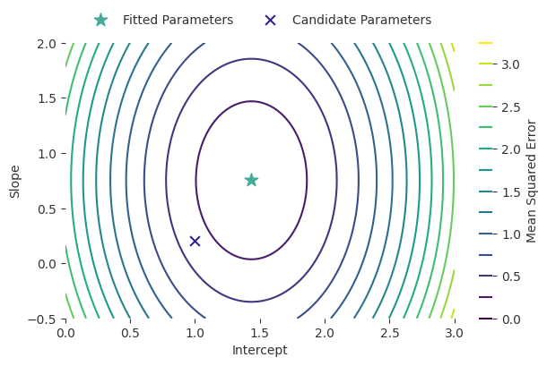

The design matrix stores a column of ones for the intercept and a column of raw readings for the slope. Check that its matrix product reproduces the fitted predictions.

X = np.column_stack([np.ones(len(x)), x])
weights = np.array([b_fit, w_fit])
assert np.allclose(X @ weights, fit)

Each point in this plot describes an entire prediction line. The fitted parameters sit at the smallest loss, and the same fitted line can be written using a design matrix. Change b and w in the first cell to move the candidate around this surface. The dataset and fitted optimum remain fixed.