Fitting a Linear Model

Suppose we have recorded delivery times for a set of trips and want to predict the time for another trip. A first model might be a line relating distance to delivery time. We will choose its slope and intercept by minimizing the average squared error, then add more features, such as traffic and departure time.

Which line best fits the recorded trips?

Predictions From Features

In supervised learning, each observed example pairs measured features with a label, the outcome we want to predict. For delivery-time prediction, the features could include trip distance, departure time, and traffic conditions when the order is placed. The label is the actual time until delivery. For spam detection, the features describe the message’s content and sender. The label records whether a person marked it as spam. Labels tell the model what to learn from past examples, but they are unavailable for a new example when its prediction is needed.

Predicting a numerical label, such as delivery time, is called regression. Predicting a category, such as spam or not spam, is called classification. We begin with regression and use a line to predict a numerical label from one feature.

For one numerical feature \(x\), a linear model predicts a label through a slope \(w\) and an intercept \(b\): \[ \widehat y=wx+b. \] The slope specifies how much the prediction changes when \(x\) increases by one unit. The intercept is the prediction at \(x=0\). The measured feature is an input. The two parameters \(w\) and \(b\) specify the rule applied to that input. Fitting means choosing their values from the observed feature-label pairs.

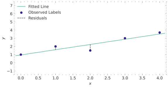
The line’s mean squared error (MSE) is the average squared vertical gap to the observations.

Changing the line can improve some predictions while worsening others. We need a single score to compare those tradeoffs across the observed examples.

Mean Squared Error

Let \((x_i,y_i)\) be the observed feature-label pairs, for \(i=1,\ldots,n\), where \(n\geq1\) is the number of examples. The residual on example \(i\) is the observed label minus the prediction: \[ r_i=y_i-(wx_i+b). \] A positive residual means the model predicted too little. A negative residual means it predicted too much. Adding signed residuals would allow overpredictions and underpredictions to cancel. Squaring each residual makes both directions costly, while making a residual twice as large cost four times as much.

The mean squared error over these \(n\) pairs is: \[ \mathcal{L}(w,b)=\frac1n\sum_{i=1}^n\bigl(y_i-wx_i-b\bigr)^2. \] A loss function assigns a cost to a prediction or a collection of predictions. Here \(\mathcal{L}\) scores the complete fitted line on the observed dataset. Dividing by \(n\) expresses an average error per example and preserves the minimizing parameters. MSE has units equal to the square of the label’s units.

The vertical segments measure differences in the predicted quantity while keeping the observed feature fixed. Their squared lengths are the terms minimized by MSE.

Choosing the Parameters

Calculus prepares us to solve optimization problems like this: derivatives tell us how a loss changes as we vary a parameter. We set the derivatives equal to zero, solve for candidate parameters, and check that they minimize the loss. Here we differentiate with respect to \(w\) and \(b\), treating the observed data as fixed.

Claim: If the observed feature takes at least two distinct values, the unique MSE-minimizing line has parameters \[ \begin{aligned} w^\star&=\frac{n\sum_{i=1}^n x_iy_i-(\sum_{i=1}^n x_i)(\sum_{i=1}^n y_i)} {n\sum_{i=1}^n x_i^2-(\sum_{i=1}^n x_i)^2},\\ b^*&=\frac{\sum_{i=1}^n y_i-w^\star\sum_{i=1}^n x_i}{n}. \end{aligned} \] Every sum runs over the \(n\) observed examples.

Proof

Let

\[ \bar x=\frac1n\sum_{i=1}^n x_i \qquad\text{and}\qquad \bar y=\frac1n\sum_{i=1}^n y_i. \]

First differentiate the loss with respect to the intercept:

\[ \frac{\partial\mathcal{L}}{\partial b} = -\frac2n\sum_{i=1}^n \bigl(y_i-wx_i-b\bigr). \]

Setting this derivative equal to zero gives

\[ b=\bar y-w\bar x. \]

Thus, for any slope \(w\), the best intercept makes the fitted line pass through \((\bar x,\bar y)\).

Substituting this intercept into the loss gives

\[ \mathcal{L}(w) = \frac1n\sum_{i=1}^n \left[ \bigl(y_i-\bar y\bigr) -w\bigl(x_i-\bar x\bigr) \right]^2. \]

Differentiating with respect to \(w\) gives

\[ \mathcal{L}'(w) = -\frac2n\sum_{i=1}^n \bigl(x_i-\bar x\bigr) \left[ \bigl(y_i-\bar y\bigr) -w\bigl(x_i-\bar x\bigr) \right]. \]

Setting this equal to zero and solving for \(w\) gives

\[ w^\star = \frac{ \sum_{i=1}^n \bigl(x_i-\bar x\bigr) \bigl(y_i-\bar y\bigr) }{ \sum_{i=1}^n\bigl(x_i-\bar x\bigr)^2 }. \]

Because at least two feature values differ, the centered sum of squares is positive. Thus

\[ \mathcal{L}''(w) = \frac2n\sum_{i=1}^n\bigl(x_i-\bar x\bigr)^2>0, \]

so \(w^\star\) is the unique minimizing slope. Its corresponding intercept is

\[ b^*=\bar y-w^\star\bar x. \]

Expanding the centered sums produces the formulas in the claim.

The denominator measures how much the feature varies. If every feature value is identical, that denominator is zero: the observations cannot distinguish a change in slope from a compensating change in intercept. Only the prediction at the shared feature value is determined, and its best value is the average observed label. More generally, among constant predictions alone, the best squared-error fit is the sample mean.

Several Features in One Matrix

Delivery-time prediction may combine distance, traffic, and departure time. For a feature vector \(\mathbf x\in\mathbb R^d\), weights \(\mathbf w\in\mathbb R^d\) produce the prediction: \[ \widehat y=\mathbf w^\top\mathbf x+b. \] Each weight multiplies one feature, and the products are added. A weight describes how the prediction changes while the other features are held fixed. Establishing a causal effect requires additional assumptions about how the data were generated.

A constant feature equal to one lets us absorb the intercept into the weight vector. For one feature, the design matrix and label vector are: \[ \mathbf X=\begin{bmatrix} 1&x_1\\ \vdots&\vdots\\ 1&x_n \end{bmatrix}, \qquad \mathbf y=\begin{bmatrix}y_1\\\vdots\\y_n\end{bmatrix}. \] Each row describes one example. Multiplying \(\mathbf X\) by \((b,w)^\top\) evaluates the line on every example at once.

From now on, let \(d\) count all feature columns, including a constant column when an intercept is used. The \(n\) rows of \(\mathbf X\in\mathbb R^{n\times d}\) contain the features, and \(\mathbf y\in\mathbb R^n\) contains the labels. The predictions and loss become: \[ \widehat{\mathbf y}=\mathbf X\mathbf w, \qquad \mathcal{L}(\mathbf w)=\frac1n\|\mathbf y-\mathbf X\mathbf w\|_2^2. \] The squared Euclidean norm sums the squared entries of the residual vector, so this is exactly the MSE already defined example by example. Fitting selects a weight vector with the smallest loss among the permitted linear predictions. This is empirical risk minimization: optimize an average loss over observed data within a chosen family of models.

Fitting a Plane

With two measured features, \(\widehat y=w_1x_1+w_2x_2+b\) describes a plane. The residuals are still vertical gaps. In the loss landscape, each point is a parameter triple \((w_1,w_2,b)\), and the transparent surfaces join choices with equal MSE.

The fitted line answers how to combine the available measurements to reduce observed squared error. Whether that rule predicts new observations accurately requires data it was not fitted on. First, the next reading develops how to find the best linear prediction when several features act together.