import numpy as np
import matplotlib.pyplot as plt

plt.style.use("../figure_style.mplstyle")

rng = np.random.default_rng(6)
temperature = rng.uniform(58, 100, 40)
x = (temperature - 79) / 21
y = 60 - 0.03 * (temperature - 85) ** 2 + rng.normal(0, 5, len(x))
grid_temperature = np.linspace(58, 100, 200)
grid_x = (grid_temperature - 79) / 21

X_linear = np.column_stack([np.ones(len(x)), x])
X_quadratic = np.column_stack([np.ones(len(x)), x, x ** 2])
grid_linear = np.column_stack([np.ones(len(grid_x)), grid_x])
grid_quadratic = np.column_stack([np.ones(len(grid_x)), grid_x, grid_x ** 2])Demo: Curves and Redundant Features
A store’s sales vary with temperature, with a possible decline in extreme heat. We use simulated sales to compare fixed feature maps and then duplicate a column. The experiment separates what the features can express from which weights express it.
Adding a Curved Feature
Predict whether adding a squared-temperature feature can increase the minimum training MSE. We express temperature as \(x=(t-79)/21\) to keep its powers on a comparable numerical scale.
Each fit changes only the available feature columns. The plotting grid lets us compare the two prediction curves between observations.
linear_weights = np.linalg.lstsq(X_linear, y, rcond=None)[0]
quadratic_weights = np.linalg.lstsq(X_quadratic, y, rcond=None)[0]
linear_mse = np.mean((y - X_linear @ linear_weights) ** 2)
quadratic_mse = np.mean((y - X_quadratic @ quadratic_weights) ** 2)
print(f"Degree 1 training MSE: {linear_mse:.3f}")
print(f"Degree 2 training MSE: {quadratic_mse:.3f}")

fig, ax = plt.subplots(figsize=(7, 3.5))
ax.scatter(temperature, y, edgecolors="none", label="Observed Sales")
ax.plot(grid_temperature, grid_linear @ linear_weights,
        linestyle="--", label="Degree 1")
ax.plot(grid_temperature, grid_quadratic @ quadratic_weights,
        label="Degree 2")
ax.set_xlabel("Temperature (°F)")
ax.set_ylabel("Sales")
ax.legend(frameon=False)
plt.show()
Degree 1 training MSE: 44.532
Degree 2 training MSE: 18.717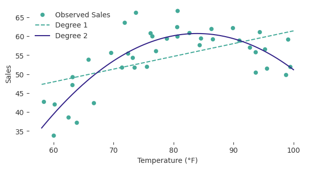
The new column permits a curved prediction while the model stays linear in its weights. The degree-two family contains every degree-one prediction, so its optimal training loss cannot be larger. np.linalg.lstsq computes a least-squares solution without explicitly inverting the normal-equation matrix.
Residual Orthogonality
The quadratic design has columns \(1,x,x^2\). Predict the inner product of each column with the fitted residual, then compare with a deliberately changed slope.
X = X_quadratic
weights = np.linalg.lstsq(X, y, rcond=None)[0]
residual = y - X @ weights
changed_weights = weights.copy()
changed_weights[1] += 2
changed_residual = y - X @ changed_weights
print("Feature-residual inner products at the fit:", np.round(X.T @ residual, 9))
print("After changing the slope:", np.round(X.T @ changed_residual, 3))
assert np.allclose(X.T @ residual, 0, atol=1e-9)
Feature-residual inner products at the fit: [-0. -0. -0.]
After changing the slope: [ -0.339 -26.737 -1.126]The fitted residual is perpendicular to every direction the existing columns can change. Changing the slope generally loses that property and increases the loss.
A Duplicate Column
A new sensor could report exactly the same measurement as an existing sensor. Predict whether adding a duplicate of \(x\) changes the fitted predictions or the number of possible weight vectors.
duplicate_scale = 1.0  # Try 2.0: the new column still adds no direction.
X_duplicate = np.column_stack([X, duplicate_scale * x])
minimum_norm = np.linalg.lstsq(X_duplicate, y, rcond=None)[0]
null_direction = np.array([0, -duplicate_scale, 0, 1])
alternative = minimum_norm + 10 * null_direction

print("Original weights:", np.round(weights, 3))
print("Minimum-norm duplicate weights:", np.round(minimum_norm, 3))
print("Alternative duplicate weights:", np.round(alternative, 3))
print(f"Minimum-norm weight length: {np.linalg.norm(minimum_norm):.3f}")
print(f"Alternative weight length: {np.linalg.norm(alternative):.3f}")
print("Maximum prediction change after duplication:",
      f"{np.max(np.abs(X_duplicate @ minimum_norm - X @ weights)):.2e}")
assert np.allclose(X_duplicate @ minimum_norm, X @ weights)
assert np.allclose(X_duplicate @ alternative, X @ weights)
assert np.linalg.norm(minimum_norm) < np.linalg.norm(alternative)
Original weights: [ 59.812 7.683 -16.329]
Minimum-norm duplicate weights: [ 59.812 3.842 -16.329 3.842]
Alternative duplicate weights: [ 59.812 -6.158 -16.329 13.842]
Minimum-norm weight length: 62.238
Alternative weight length: 63.825
Maximum prediction change after duplication: 5.68e-14The duplicate adds a parameter but no reachable prediction direction. All displayed duplicate-model weights make the same predictions. The pseudoinverse chooses the shortest weight vector in those coordinates. Change duplicate_scale to see how that chosen vector changes even though the fitted predictions remain the same.