Least Squares
Last time, we fit a line by choosing a slope and intercept. With several features, we have more weights to choose, but the goal is the same: minimize squared training error. Some labels may be impossible to fit exactly, and several weight vectors may give the same best fit.
We will use the singular value decomposition to separate the error into directions we can fit and a part we cannot change, then connect the resulting solution to the gradient.
Residual and Column Space
Let \(\mathbf X\in\mathbb R^{n\times d}\) contain \(d\) features for each of \(n\geq1\) training examples, with one example per row, and let \(\mathbf y\in\mathbb R^n\) contain the labels. Using weights \(\mathbf w\in\mathbb R^d\), we predict \(\mathbf X\mathbf w\) and minimize the mean squared error: \[ \mathcal L(\mathbf w)=\frac1n\|\mathbf X\mathbf w-\mathbf y\|_2^2. \] The features can include nonlinear functions of the original inputs, such as their squares. We will return to polynomial features at the end; the model is linear in the weights throughout.
Each feature column lists that feature’s values across all training examples. The prediction vector is a weighted combination of these columns: \[ \mathbf X\mathbf w=\sum_{j=1}^d w_j[\mathbf X]_{:,j}. \] The column space of \(\mathbf X\) consists of all these combinations, so it contains every prediction vector our model can produce. The weights live in parameter space \(\mathbb R^d\), while the labels and predictions live in training-prediction space \(\mathbb R^n\).
The singular value decomposition (SVD) gives orthonormal directions in each space. Write \[ \mathbf X=\mathbf U\boldsymbol\Sigma\mathbf V^\top =\sum_{i=1}^r\sigma_i\mathbf u_i\mathbf v_i^\top, \qquad r=\operatorname{rank}(\mathbf X). \] Here \(\mathbf U\in\mathbb R^{n\times r}\) and \(\mathbf V\in\mathbb R^{d\times r}\) have orthonormal columns \(\mathbf u_i\) and \(\mathbf v_i\), and \(\boldsymbol\Sigma\in\mathbb R^{r\times r}\) contains the positive singular values, ordered as \(\sigma_1\ge\cdots\ge\sigma_r>0\) when \(r>0\). Their indices run from \(1\) to \(r\). An empty sum is zero, so the decomposition also covers \(\mathbf X=\mathbf0\) with \(r=0\). The map sends each parameter direction to its matching prediction direction: \[ \mathbf X\mathbf v_i=\sigma_i\mathbf u_i. \] Thus the \(\mathbf u_i\) span the column space.
Every weight vector can be decomposed as \[ \mathbf w=\sum_{i=1}^r c_i\mathbf v_i+\mathbf w_\perp, \] where \(c_i=\mathbf v_i^\top\mathbf w\) and \(\mathbf w_\perp\) is perpendicular to every \(\mathbf v_i\). The SVD gives \(\mathbf X\mathbf w_\perp=\mathbf0\). These components of the weights have no effect on the training predictions. Similarly, decompose the labels as \[ \mathbf y=\sum_{i=1}^r(\mathbf u_i^\top\mathbf y)\mathbf u_i+\mathbf y_\perp, \] where \(\mathbf y_\perp\) is perpendicular to every \(\mathbf u_i\). This part of the labels lies outside the predictions our model can produce.
Applying \(\mathbf X\) to the weights and subtracting the labels gives \[ \mathbf X\mathbf w-\mathbf y =\sum_{i=1}^r(\sigma_i c_i-\mathbf u_i^\top\mathbf y)\mathbf u_i-\mathbf y_\perp. \] The directions in this expression are perpendicular. By the Pythagorean theorem, the training error separates into \[ \mathcal L(\mathbf w) =\frac1n\sum_{i=1}^r(\sigma_i c_i-\mathbf u_i^\top\mathbf y)^2 +\frac1n\|\mathbf y_\perp\|_2^2. \] We can make each term in the sum zero by choosing its coefficient \(c_i\). The remaining error is fixed by the features and labels.
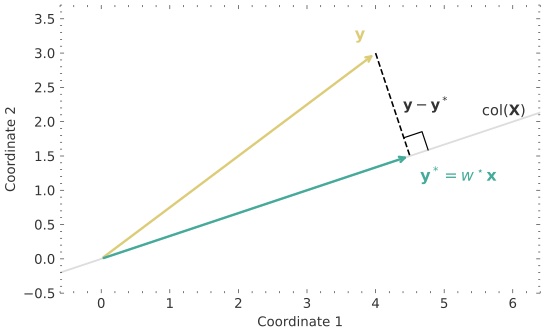
At the minimum, the fitted prediction is the orthogonal projection of \(\mathbf y\) onto the column space: \[ \widehat{\mathbf y}=\sum_{i=1}^r(\mathbf u_i^\top\mathbf y)\mathbf u_i. \] The residual \(\mathbf y-\widehat{\mathbf y}=\mathbf y_\perp\) is perpendicular to every reachable prediction. With one nonzero feature column \(\mathbf x\), the reachable predictions \(w\mathbf x\) form a line.
Prediction Space
Loss Landscape
Optimal Weights
The error decomposition tells us exactly which coefficients to choose: \[ c_i=\frac{\mathbf u_i^\top\mathbf y}{\sigma_i}. \] Each coefficient matches the labels in one prediction direction. The component \(\mathbf w_\perp\) is still free because it leaves all training predictions unchanged. The vectors satisfying \(\mathbf X\mathbf w_\perp=\mathbf0\) form the null space of \(\mathbf X\).
Claim: Every least-squares minimizer has the form \[ \mathbf w=\sum_{i=1}^r\frac{\mathbf u_i^\top\mathbf y}{\sigma_i}\mathbf v_i+\mathbf w_\perp, \qquad \mathbf X\mathbf w_\perp=\mathbf0. \]
Proof
The loss is a sum of nonnegative squared terms plus the fixed term \(\|\mathbf y_\perp\|_2^2/n\). Substituting the proposed coefficients makes every squared term zero, so these weights achieve the smallest possible loss. Conversely, attaining that loss requires each squared term to vanish. Because \(\sigma_i>0\), this fixes each \(c_i\) to the displayed value and leaves only \(\mathbf w_\perp\) free.
The fit is unique exactly when \(r=d\), since then the null space contains only zero. Every label vector can be fitted exactly when \(r=n\), since then the column space fills \(\mathbb R^n\). Under the full-rank assumption \(r=\min(n,d)\), these facts give three cases:
- If \(d<n\), the fit is unique, but its training error can be positive.
- If \(d=n\), the fit is unique and fits every label exactly.
- If \(d>n\), infinitely many weight vectors fit every label exactly.
Repeated or linearly dependent features can reduce the rank below \(\min(n,d)\); the same decomposition still applies.
When several weights give the same fit, choosing the one with the smallest norm sets every undetermined component to zero. Define the pseudoinverse by reversing the positive singular values: \[ \mathbf X^+=\sum_{i=1}^r\frac1{\sigma_i}\mathbf v_i\mathbf u_i^\top =\mathbf V\boldsymbol\Sigma^{-1}\mathbf U^\top\in\mathbb R^{d\times n}. \] It takes each label component along \(\mathbf u_i\), divides it by \(\sigma_i\), and places it along \(\mathbf v_i\).
Claim: The unique minimum-norm least-squares fit is \[ \widehat{\mathbf w}=\mathbf X^+\mathbf y. \]
Proof
The previous claim shows that \(\widehat{\mathbf w}\) minimizes the loss and every other minimizer is \(\widehat{\mathbf w}+\mathbf w_\perp\). Since \(\widehat{\mathbf w}\) is a combination of the \(\mathbf v_i\), it is perpendicular to \(\mathbf w_\perp\). Therefore \[ \|\widehat{\mathbf w}+\mathbf w_\perp\|_2^2 =\|\widehat{\mathbf w}\|_2^2+\|\mathbf w_\perp\|_2^2. \] The norm is uniquely minimized by setting \(\mathbf w_\perp=\mathbf0\).
For \(\mathbf X=\mathbf0\), the sums are empty and the minimum-norm fit is \(\widehat{\mathbf w}=\mathbf0\).
Computing the Gradient
We found the optimal weights by separating the training error into independent terms. To find them through repeated updates, we need the gradient. Let \(\mathbf r=\mathbf y-\mathbf X\mathbf w\) be the residual vector. Increasing \(w_j\) changes prediction \(i\) at rate \([\mathbf X]_{i,j}\), so the chain rule gives \[ \frac{\partial\mathcal L}{\partial w_j} =\frac2n\sum_{i=1}^n r_i\frac{\partial r_i}{\partial w_j} =-\frac2n\sum_{i=1}^n[\mathbf X]_{i,j}r_i. \] The sum is entry \(j\) of \(\mathbf X^\top\mathbf r\). Collecting the partial derivatives into the gradient gives \[ \nabla\mathcal L(\mathbf w)=\frac2n\mathbf X^\top(\mathbf X\mathbf w-\mathbf y). \]
Setting the gradient to zero gives the normal equations: \[ \mathbf X^\top(\mathbf X\mathbf w-\mathbf y)=\mathbf0 \quad\Longleftrightarrow\quad \mathbf X^\top\mathbf X\mathbf w=\mathbf X^\top\mathbf y. \] The first equality says that the residual is perpendicular to every feature column. This is exactly the projection condition: the remaining error lies in the directions our features cannot fit. It also suffices for a global minimum, because any weight change \(\mathbf h\in\mathbb R^d\) then satisfies \[ \mathcal L(\mathbf w+\mathbf h) =\mathcal L(\mathbf w)+\frac1n\|\mathbf X\mathbf h\|_2^2 \ge\mathcal L(\mathbf w). \] The cross term vanishes because \(\mathbf X^\top\mathbf r=\mathbf0\).
In SVD coordinates, the derivative with respect to each coefficient is \[ \frac{\partial\mathcal L}{\partial c_i} =\frac2n\sigma_i(\sigma_i c_i-\mathbf u_i^\top\mathbf y). \] Its zero gives the coefficient we already derived. The factor \(\sigma_i^2\) determines how quickly this derivative changes as we move \(c_i\); in the next reading, it will determine how gradient descent progresses along each direction.
When the columns are independent, \(\mathbf X^\top\mathbf X\) is invertible: for every nonzero \(\mathbf h\), we have \(\mathbf h^\top\mathbf X^\top\mathbf X\mathbf h=\|\mathbf X\mathbf h\|_2^2>0\). The normal equations give another expression for the unique fit: \[ \widehat{\mathbf w}=(\mathbf X^\top\mathbf X)^{-1}\mathbf X^\top\mathbf y. \] Building \(\mathbf X^\top\mathbf X\) costs \(O(nd^2)\), and solving this dense linear system costs \(O(d^3)\). These costs motivate the iterative methods we study next. Problem 6 uses the linear dependence of fitted predictions on the labels to evaluate each observation with its label omitted, without fitting a separate model each time.
Curved Predictions From Fixed Features
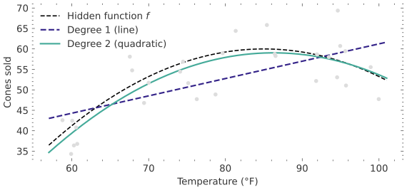
A straight line can miss a curved calibration relationship even when its weights are fitted perfectly. We can change which predictions are reachable by changing the feature columns. A feature map \(\phi\) converts a raw measurement into the \(d\) features supplied to the linear model: \[ f(x)=\mathbf w^\top\phi(x), \qquad \phi(x)\in\mathbb R^d. \] For one scalar measurement, choose \(\phi(x)=(1,x,x^2)^\top\). The resulting prediction is: \[ f(x)=w_0+w_1x+w_2x^2. \] It is curved as a function of the raw measurement but linear in the three unknown weights. The design matrix gains a column of squared measurements, so the same projection and solver apply.
A store’s sales may rise with temperature over one range and fall in extreme heat. A line can only increase, decrease, or stay constant. A quadratic feature permits a turning point.
Let \(x\) denote centered, scaled temperature and \(y\) sales in scaled units.
Prediction Space
The feature map chooses the possible shapes before the weights are fitted. Adding a column cannot worsen the minimum training loss because every old prediction is still available by setting its new weight to zero. It need not improve predictions on fresh data: a new direction can fit accidental label variation as well as a persistent relationship.
Least squares finds the reachable prediction closest to the labels. A more elaborate feature map changes the reachable space. An iterative solver changes how we search for that same closest point.