Demo: Feature Units and Training Speed

We fit a two-feature calibration model to a fixed set of observations. Both versions of the model can express exactly the same predictions. One uses raw feature units. The other divides each feature by its length.

Two Coordinate Systems

Predict which design will have the larger ratio between the steepest and shallowest loss curvatures. scale changes the units of the second feature while preserving its contribution to the labels.

import numpy as np
import matplotlib.pyplot as plt

plt.style.use("../figure_style.mplstyle")

rng = np.random.default_rng(7)
n = 200
features = rng.normal(size=(n, 2))
y = features @ np.array([1.0, 1.0]) + rng.normal(0, 0.2, n)
scale = 20.0  # Change this and rerun all cells.
X = features.copy()
X[:, 1] *= scale
column_lengths = np.linalg.norm(X, axis=0)
X_scaled = X / column_lengths
for label, design in [("Raw", X), ("Scaled", X_scaled)]:
    H = 2 * design.T @ design / n
    eigenvalues = np.linalg.eigvalsh(H)
    print(f"{label} Hessian condition number: {eigenvalues[-1] / eigenvalues[0]:.2f}")

Raw Hessian condition number: 410.91
Scaled Hessian condition number: 1.29

Changing feature units changes curvature in parameter coordinates. It preserves the column space, so both models have the same least-squares prediction.

Equal Iteration Budgets

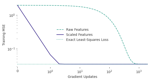
Each run starts at zero and gets 2,000 full-gradient updates. We give each coordinate system its own optimal fixed step \(2/(\lambda_{\max}+\lambda_{\min})\). Each system therefore uses its own best fixed step size. Predict whether either run can beat the exact least-squares loss.

steps = 2000
reference_weights = np.linalg.lstsq(X, y, rcond=None)[0]
best_loss = np.mean((X @ reference_weights - y) ** 2)

fig, ax = plt.subplots(figsize=(7, 3.5))
for label, design, linestyle in [
    ("Raw Features", X, "--"),
    ("Scaled Features", X_scaled, "-"),
]:
    H = 2 * design.T @ design / n
    eigenvalues = np.linalg.eigvalsh(H)
    alpha = 2 / (eigenvalues[0] + eigenvalues[-1])
    weights = np.zeros(2)
    losses = [np.mean((design @ weights - y) ** 2)]

    for _ in range(steps):
        prediction_error = design @ weights - y
        gradient = 2 * design.T @ prediction_error / n
        weights = weights - alpha * gradient
        loss = np.mean((design @ weights - y) ** 2)
        losses.append(loss)

    ax.plot(losses, linestyle=linestyle, label=label)
    print(f"{label}: step {alpha:.4g}, final MSE {losses[-1]:.6f}")
    assert min(losses) >= best_loss - 1e-10
ax.axhline(best_loss, linestyle=":", label="Exact Least-Squares Loss")
ax.set_xscale("symlog", linthresh=1)
ax.set_yscale("log")
ax.set_xlim(0, steps)
ax.set_xlabel("Gradient Updates")
ax.set_ylabel("Training MSE")
ax.legend(frameon=False)
plt.show()

Raw Features: step 0.002875, final MSE 0.034768
Scaled Features: step 100, final MSE 0.034768

The reference line is the smallest loss either coordinate system can reach. The scaled features let a single learning rate make progress in both directions. The raw features require a compromise.

The Predicted Contraction

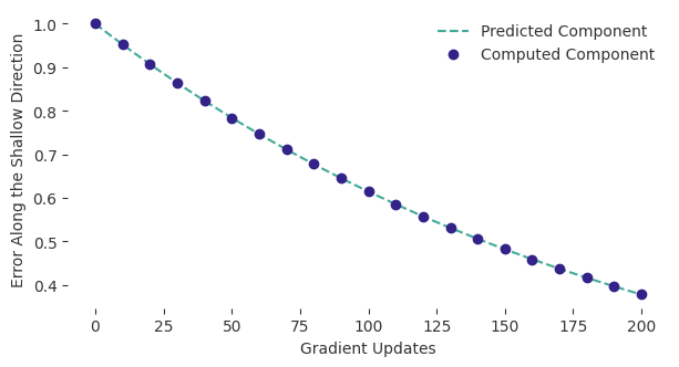
The reading predicts that an error component along an eigenvector changes by \(1-\alpha\lambda\) each step. We start with an error only in the shallowest direction and compare that exact prediction with the updates.

H = 2 * X.T @ X / n
eigenvalues, eigenvectors = np.linalg.eigh(H)
alpha = 2 / (eigenvalues[0] + eigenvalues[-1])
shallow_direction = eigenvectors[:, 0]
weights = reference_weights + shallow_direction
components = []
for _ in range(201):
    components.append(shallow_direction @ (weights - reference_weights))
    gradient = 2 * X.T @ (X @ weights - y) / n
    weights = weights - alpha * gradient
predicted = (1 - alpha * eigenvalues[0]) ** np.arange(201)
assert np.allclose(components, predicted, atol=1e-10)
fig, ax = plt.subplots(figsize=(7, 3.5))
ax.plot(predicted, linestyle="--", label="Predicted Component")
ax.plot(np.arange(0, 201, 10), np.array(components)[::10], marker="o", linestyle="none", label="Computed Component")
ax.set_xlabel("Gradient Updates")
ax.set_ylabel("Error Along the Shallow Direction")
ax.legend(frameon=False)
plt.show()

The numerical updates agree with the predicted geometric contraction. Changing scale changes that factor while keeping the observations and attainable predictions fixed. Scaling can remove a difference in units. Nearly parallel feature columns can still leave a shallow direction.