Demo: Selecting a Model on New Data

We simulate a curved calibration relationship and fit polynomials of different degrees. Training, validation, and test labels use independent noise. The training inputs are fixed calibration settings. Validation and test inputs cover the same interval.

Training and Validation

Predict which loss is guaranteed not to increase as polynomial degree grows. The columns of a degree-\(k\) design matrix are \(1,x,x^2,\ldots,x^k\). The polynomial_features function builds those columns directly.

import numpy as np
import matplotlib.pyplot as plt

plt.style.use("../figure_style.mplstyle")

rng = np.random.default_rng(8)
sigma = 0.3
n_train = 24
x_train = np.linspace(-1, 1, n_train)
x_val = rng.uniform(-1, 1, 200)

def conditional_mean(x):
    return 1 + x - 1.5 * x ** 2

def polynomial_features(x, degree):
    columns = []
    for power in range(degree + 1):
        columns.append(x ** power)
    return np.column_stack(columns)

Each degree uses the same training and validation observations. Predict which score will prefer the most flexible model.

y_train = conditional_mean(x_train) + rng.normal(0, sigma, n_train)
y_val = conditional_mean(x_val) + rng.normal(0, sigma, len(x_val))
degrees = np.arange(10)
train_mse = []
val_mse = []
fitted_weights = []
for degree in degrees:
    X_train = polynomial_features(x_train, degree)
    X_val = polynomial_features(x_val, degree)
    weights = np.linalg.lstsq(X_train, y_train, rcond=None)[0]
    fitted_weights.append(weights)
    train_mse.append(np.mean((X_train @ weights - y_train) ** 2))
    val_mse.append(np.mean((X_val @ weights - y_val) ** 2))
assert np.all(np.diff(train_mse) <= 1e-10)

fig, ax = plt.subplots(figsize=(7, 3.5))
ax.plot(degrees, train_mse, marker="s", linestyle="--", label="Training")
ax.plot(degrees, val_mse, marker="o", label="Validation")
ax.axhline(sigma ** 2, linestyle=":", label="Population Noise Floor")
ax.set_xlabel("Polynomial Degree")
ax.set_ylabel("Mean Squared Error")
ax.legend(frameon=False)
plt.show()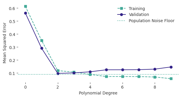

Training MSE cannot rise because the polynomial families are nested. Validation MSE has no such guarantee. The noise floor is the expected error from fresh-label noise. A finite sample’s measured MSE can fall below it.

One Test of the Selected Model

Choose the degree using validation error, freeze that choice, and only then generate the test labels. Predict whether the test score must equal the winning validation score.

best_index = np.argmin(val_mse)
chosen_degree = degrees[best_index]
weights = fitted_weights[best_index]
x_test = rng.uniform(-1, 1, 4000)
y_test = conditional_mean(x_test) + rng.normal(0, sigma, len(x_test))
X_test = polynomial_features(x_test, chosen_degree)
test_mse = np.mean((X_test @ weights - y_test) ** 2)
print(f"Selected degree: {chosen_degree}")
print(f"Winning validation MSE: {val_mse[best_index]:.4f}")
print(f"Untouched test MSE: {test_mse:.4f}")

Selected degree: 2
Winning validation MSE: 0.0973
Untouched test MSE: 0.0963

Selection used the validation scores, so evaluating the selected model requires a separate test set. The test score evaluates the selected rule on untouched examples. If we change the model after seeing this test result, that set no longer supplies an untouched test.

Repeated Calibration Runs

Bias and variance concern the fitting procedure across new training labels. Hold the inputs and polynomial degrees fixed, redraw the training noise, and inspect the resulting predictions. Predict what increasing n_train will do to the variability of flexible fits.

repetitions = 300
x_grid = np.linspace(-1, 1, 201)
mean_train = conditional_mean(x_train)
mean_grid = conditional_mean(x_grid)

# Reuse these training sets so each degree sees the same noise.
training_sets = []
for _ in range(repetitions):
    labels = mean_train + rng.normal(0, sigma, n_train)
    training_sets.append(labels)

bias_squared = []
variance = []
expected_error = []
for degree in degrees:
    X_train = polynomial_features(x_train, degree)
    X_grid = polynomial_features(x_grid, degree)
    predictions = []
    for labels in training_sets:
        weights = np.linalg.lstsq(X_train, labels, rcond=None)[0]
        predictions.append(X_grid @ weights)
    predictions = np.array(predictions)

    # Rows are fitted models; columns are inputs on the plotting grid.
    average_prediction = predictions.mean(axis=0)
    bias_squared.append(np.mean((average_prediction - mean_grid) ** 2))
    variance.append(np.mean(predictions.var(axis=0)))
    expected_error.append(np.mean((predictions - mean_grid) ** 2) + sigma ** 2)

bias_squared = np.array(bias_squared)
variance = np.array(variance)
expected_error = np.array(expected_error)
assert np.allclose(expected_error, bias_squared + variance + sigma ** 2)

The next plot averages over the input grid. Compare the growth in variance with the reduction in squared bias as degree increases.

fig, ax = plt.subplots(figsize=(7, 3.5))
ax.plot(degrees, bias_squared, marker="s", linestyle="--", label="Squared Bias")
ax.plot(degrees, variance, marker="o", label="Variance")
ax.plot(degrees, expected_error, marker="^", linestyle="-.", label="Fresh-Label Error")
ax.axhline(sigma ** 2, linestyle=":", label="Irreducible Noise")
ax.set_xlabel("Polynomial Degree")
ax.set_ylabel("Error Averaged Over the Input Grid")
ax.legend(frameon=False)
plt.show()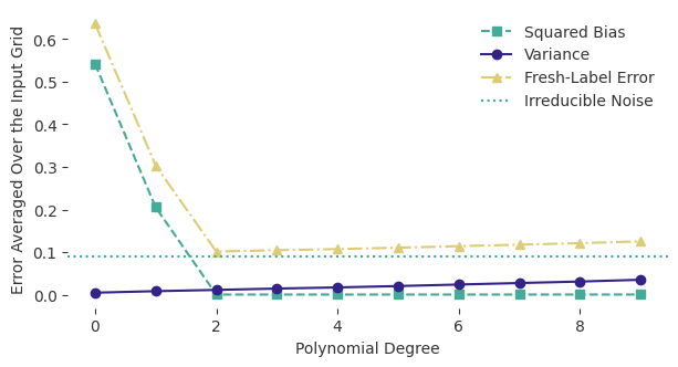

These estimates average over 300 fitted models and a fixed input grid. For each fit, the fresh-label error integrates out the independent label noise exactly by adding \(\sigma^2\). The decomposition into squared bias, variance, and noise holds exactly for the empirical distribution of these repeated fits. The estimates of the full training-distribution quantities still have Monte Carlo error. Increase n_train in the first cell and rerun to compare the same degree range with more calibration observations.