Demo: One Faulty Sensor, Two Losses

Several sensors measure one common quantity, so our prediction model is a constant \(c\). We hold the trustworthy readings fixed and move one corrupted reading. Gaussian and Laplace observation models yield squared and absolute losses, respectively.

Fitted Constants

Predict which estimate will move farther when the corrupted reading is increased.

import numpy as np
import matplotlib.pyplot as plt

plt.style.use("../figure_style.mplstyle")

rng = np.random.default_rng(9)
clean = rng.normal(10, 1, 30)
corrupted = 25.0  # Change this and rerun.
y = np.append(clean, corrupted)

Compare the two fitted constants with the sensor readings.

fig, ax = plt.subplots(figsize=(7, 2.8))
ax.scatter(clean, np.zeros_like(clean), edgecolors="none", label="Trustworthy Readings")
ax.scatter([corrupted], [0], marker="x", label="Corrupted Reading")
ax.axvline(y.mean(), label="Squared-Loss Fit: Mean")
ax.axvline(np.median(y), linestyle="--", label="Absolute-Loss Fit: Median")
ax.set_xlabel("Sensor Reading")
ax.set_yticks([])
ax.set_ylim(-0.1, 0.5)
ax.legend(frameon=False, ncol=2, loc="lower center", bbox_to_anchor=(0.5, 1.02))
plt.show()
print(f"Mean: {y.mean():.3f}, median: {np.median(y):.3f}")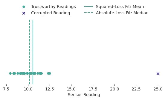

Mean: 10.579, median: 10.186

The mean depends on the magnitude of every observation. The median depends on the ordering around the middle.

Likelihood and Loss Give the Same Ranking

For fixed Gaussian standard deviation \(\sigma\) and Laplace scale \(b\), negative log likelihood is a positive multiple of the corresponding summed loss plus a constant. Predict whether removing the constants can move either minimum.

candidates = np.linspace(min(8, y.mean() - 2), max(13, y.mean() + 2), 500)
mse = []
mae = []
for c in candidates:
    residuals = y - c
    mse.append(np.mean(residuals ** 2))
    mae.append(np.mean(np.abs(residuals)))
mse = np.array(mse)
mae = np.array(mae)
sigma, b = 1.0, 1.0
nll_gaussian = len(y) * (0.5 * np.log(2 * np.pi * sigma ** 2) + mse / (2 * sigma ** 2))
nll_laplace = len(y) * (np.log(2 * b) + mae / b)
assert np.argmin(nll_gaussian) == np.argmin(mse)
assert np.argmin(nll_laplace) == np.argmin(mae)

The two losses have different units. Compare their minimizer locations.

fig, axes = plt.subplots(1, 2, figsize=(8, 3.4))
for ax, loss, center, title, ylabel in [
    (axes[0], mse, y.mean(), "Gaussian Model", "Mean Squared Error"),
    (axes[1], mae, np.median(y), "Laplace Model", "Mean Absolute Error")]:
    ax.plot(candidates, loss, label="Empirical Loss")
    ax.axvline(center, linestyle="--", label="Exact Minimizer")
    ax.set_title(title)
    ax.set_xlabel("Constant Prediction")
    ax.set_ylabel(ylabel)
fig.legend(*axes[0].get_legend_handles_labels(), loc="upper center",
           bbox_to_anchor=(0.5, 1.15), ncol=2)
fig.tight_layout()
plt.show()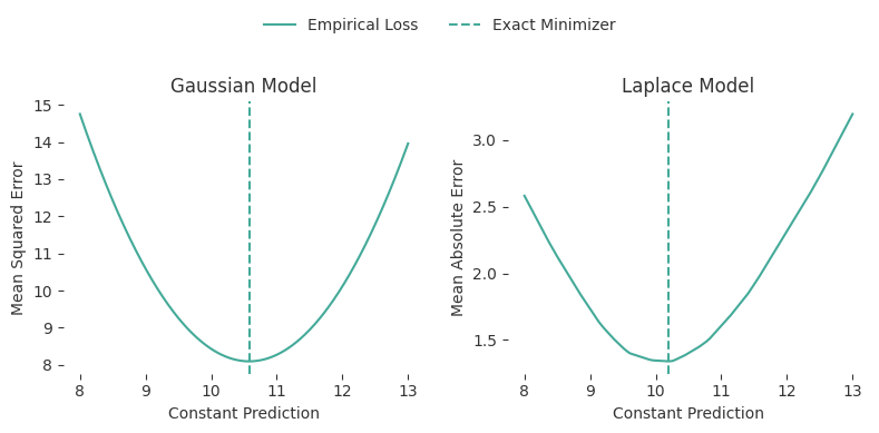

The minimum locations agree with the mean and median derived in the reading. The losses have different units. Compare the fitted centers using a common evaluation criterion.

Influence of One Observation

Hold the clean readings fixed and move only the corrupted value. Predict the shape of each fitted-constant path before plotting it.

corrupted_values = np.linspace(-20, 50, 200)
means = []
medians = []
for value in corrupted_values:
    readings = np.append(clean, value)
    means.append(readings.mean())
    medians.append(np.median(readings))
predicted_mean = (clean.sum() + corrupted_values) / (len(clean) + 1)
assert np.allclose(means, predicted_mean)

Compare how far each fitted constant moves when one reading changes.

fig, ax = plt.subplots(figsize=(7, 3.5))
ax.plot(corrupted_values, means, label="Squared-Loss Fit")
ax.plot(corrupted_values, medians, linestyle="--", label="Absolute-Loss Fit")
ax.axhline(clean.mean(), linestyle=":", label="Mean of Trustworthy Readings")
ax.set_xlabel("Corrupted Reading")
ax.set_ylabel("Fitted Constant")
ax.legend(frameon=False)
plt.show()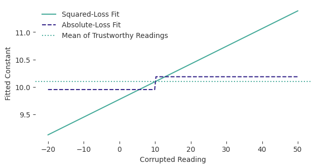

The mean moves linearly with the corrupted reading, with slope \(1/n\). The median becomes insensitive to further movement once the corrupted reading is beyond the middle observations. This experiment tests sensitivity to one arbitrary corruption. Accuracy under other noise distributions requires a separate comparison. Change corrupted to inspect the residuals and losses at another point along these paths.