Demo: The Overfitting U-Curve

Back in the Regression lecture, a 13-parameter wiggle threaded perfectly through a month of ice-cream data, then fell apart on a fresh month. Today we hold out a validation set properly and watch the same story play out, degree by degree, instead of relying on one lucky (or unlucky) comparison.

import warnings
import numpy as np
import matplotlib.pyplot as plt
import scienceplots

warnings.filterwarnings("ignore", message="The fit may be poorly conditioned")
plt.style.use(["science", "no-latex"])
TEAL, CARDINAL, GRAY = "#009090", "#9c1b33", "#c9c9c9"
rng = np.random.default_rng(9)

sigma = 5
hidden_f = lambda t: 60 - 0.03 * (t - 85) ** 2

n_train, n_val = 15, 60
temps_train = rng.uniform(58, 100, size=n_train)
sales_train = hidden_f(temps_train) + rng.normal(0, sigma, size=n_train)
temps_val = rng.uniform(58, 100, size=n_val)
sales_val = hidden_f(temps_val) + rng.normal(0, sigma, size=n_val)

print(f"training on {n_train} days, validating on {n_val} fresh days")

training on 15 days, validating on 60 fresh days

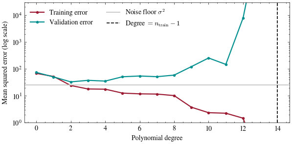
Fit a polynomial of each degree \(0, 1, 2, \ldots\) to the training days only, and score it on both sets.

degrees = np.arange(0, n_train)
train_errs, val_errs = [], []
for k in degrees:
    w = np.polynomial.Polynomial.fit(temps_train, sales_train, k)
    train_errs.append(np.mean((w(temps_train) - sales_train) ** 2))
    val_errs.append(np.mean((w(temps_val) - sales_val) ** 2))

fig, ax = plt.subplots(figsize=(7, 3.2))
ax.plot(degrees, train_errs, color=CARDINAL, linewidth=1.6, marker="o", markersize=3, label="Training error")
ax.plot(degrees, val_errs, color=TEAL, linewidth=1.6, marker="o", markersize=3, label="Validation error")
ax.axhline(sigma ** 2, color=GRAY, linewidth=1.4, label="Noise floor $\\sigma^2$")
ax.axvline(n_train - 1, color="black", linestyle="--", linewidth=1.2, label="Degree $= n_{\\mathrm{train}}-1$")
ax.set_yscale("log")
ax.set_ylim(1, 3e4)
ax.set_xlabel("Polynomial degree")
ax.set_ylabel("Mean squared error (log scale)")
ax.legend(frameon=False, loc="upper left", ncol=2)
plt.show()

best_degree = degrees[np.argmin(val_errs)]
print(f"best degree by validation error: {best_degree}  (the hidden function is degree 2)")
print(f"  training error there: {train_errs[best_degree]:.1f}, validation error there: {val_errs[best_degree]:.1f}")

best degree by validation error: 2  (the hidden function is degree 2)
  training error there: 24.1, validation error there: 32.8

Training error never goes back up, exactly the claim we proved in class, and past degree 2 it drops below the gray noise floor \(\sigma^2 = 25\), which no error on fresh data can do. Each added parameter lets the fit absorb more of the training noise. Validation error bottoms out near the true degree of 2, just above the floor, and then climbs. Past degree 12 the training error approaches zero while the validation error exceeds the plot’s range: at \(\text{degree} = n_{\text{train}} - 1\) there is one parameter per training day, and the fit interpolates the noise exactly.

Increase the training set

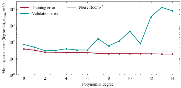
More data should let a higher-degree model generalize before it starts overfitting. Try n_train_new = 60 below, then try 25.

n_train_new = 60    # change me!

temps_train2 = rng.uniform(58, 100, size=n_train_new)
sales_train2 = hidden_f(temps_train2) + rng.normal(0, sigma, size=n_train_new)

degrees2 = np.arange(0, min(n_train_new, n_train))
train_errs2, val_errs2 = [], []
for k in degrees2:
    w = np.polynomial.Polynomial.fit(temps_train2, sales_train2, k)
    train_errs2.append(np.mean((w(temps_train2) - sales_train2) ** 2))
    val_errs2.append(np.mean((w(temps_val) - sales_val) ** 2))

fig, ax = plt.subplots(figsize=(7, 3.2))
ax.plot(degrees2, train_errs2, color=CARDINAL, linewidth=1.6, marker="o", markersize=3, label="Training error")
ax.plot(degrees2, val_errs2, color=TEAL, linewidth=1.6, marker="o", markersize=3, label="Validation error")
ax.axhline(sigma ** 2, color=GRAY, linewidth=1.4, label="Noise floor $\\sigma^2$")
ax.set_yscale("log")
ax.set_ylim(1, 3e4)
ax.set_xlabel("Polynomial degree")
ax.set_ylabel(f"Mean squared error (log scale), $n_\\mathrm{{train}}={n_train_new}$")
ax.legend(frameon=False, loc="upper left", ncol=2)
plt.show()

Overfitting depends on model capacity relative to the amount of training data. The same degree-6 polynomial that is already fitting noise on 15 days sits near the noise floor on 60. Next lecture applies the same train/validation discipline to classification.