Demo: Gradient Descent on MNIST

Today’s labels are categorical rather than real: MNIST handwritten digits, \(0\) through \(9\). We build the softmax and cross-entropy machinery from the reading by hand, then fit it with plain gradient descent because the weights have no closed-form solution.

import numpy as np
import matplotlib.pyplot as plt
import scienceplots
from matplotlib.colors import LinearSegmentedColormap
from sklearn.datasets import fetch_openml

plt.style.use(["science", "no-latex"])
TEAL, CARDINAL, GRAY = "#009090", "#9c1b33", "#c9c9c9"
CARDINAL_TEAL = LinearSegmentedColormap.from_list("cardinal_teal", [CARDINAL, "white", TEAL])
rng = np.random.default_rng(10)

X_all, y_all = fetch_openml("mnist_784", version=1, return_X_y=True, as_frame=False, parser="auto")
y_all = y_all.astype(int)

# subsample for a demo that trains in seconds, not minutes
idx = rng.choice(len(X_all), size=6000, replace=False)
X_all, y_all = X_all[idx], y_all[idx]
X_all = X_all / 255.0                      # pixels to [0, 1]
X_all = np.column_stack([X_all, np.ones(len(X_all))])   # fold in the bias column

n_train = 5000
X_train, y_train = X_all[:n_train], y_all[:n_train]
X_val, y_val = X_all[n_train:], y_all[n_train:]
print(f"training on {n_train} digits, validating on {len(X_val)}")

training on 5000 digits, validating on 1000

Build the one-hot labels, and implement the gradient exactly as derived in lecture: \(\nabla_{\mathbf{z}} \ell = \mathbf{p} - \mathbf{y}\), chained through \(\mathbf{z} = \mathbf{X}\mathbf{W}\) to give \(\frac{1}{n}\mathbf{X}^\top(\mathbf{P} - \mathbf{Y})\).

k = 10  # digit classes
d = X_train.shape[1]

def one_hot(y, k):
    Y = np.zeros((len(y), k))
    Y[np.arange(len(y)), y] = 1
    return Y

Y_train = one_hot(y_train, k)
Y_val = one_hot(y_val, k)

def softmax(Z):
    Z = Z - Z.max(axis=1, keepdims=True)   # for numerical stability; doesn't change the output
    expZ = np.exp(Z)
    return expZ / expZ.sum(axis=1, keepdims=True)

def cross_entropy(P, Y):
    return -np.mean(np.sum(Y * np.log(P + 1e-12), axis=1))

def accuracy(P, y):
    return np.mean(P.argmax(axis=1) == y)

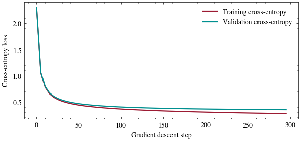
Train for \(300\) gradient steps at \(\alpha = 0.5\) starting from \(\mathbf{W}^{(0)} = \mathbf{0}\), tracking both losses as we go.

W = np.zeros((d, k))
alpha = 0.5
n_steps = 300

steps, train_losses, val_losses, val_accs = [], [], [], []
for t in range(n_steps):
    P_train = softmax(X_train @ W)

    if t % 5 == 0:   # both scores measured at the same weights, before the step
        steps.append(t)
        train_losses.append(cross_entropy(P_train, Y_train))
        P_val = softmax(X_val @ W)
        val_losses.append(cross_entropy(P_val, Y_val))
        val_accs.append(accuracy(P_val, y_val))

    grad = X_train.T @ (P_train - Y_train) / n_train      # softmax minus one-hot, averaged
    W -= alpha * grad

fig, ax = plt.subplots(figsize=(7, 3))
ax.plot(steps, train_losses, color=CARDINAL, linewidth=1.6, label="Training cross-entropy")
ax.plot(steps, val_losses, color=TEAL, linewidth=1.6, label="Validation cross-entropy")
ax.set_xlabel("Gradient descent step")
ax.set_ylabel("Cross-entropy loss")
ax.legend(frameon=False)
plt.show()

print(f"final validation accuracy: {accuracy(softmax(X_val @ W), y_val):.1%}")

final validation accuracy: 90.9%

The validation loss remains above the training loss: we are fitting \(785 \times 10 = 7{,}850\) parameters to \(5{,}000\) points, so the fitted weights absorb some training noise.

Inspect the learned class templates

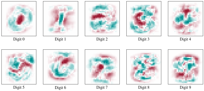
Each column of \(\mathbf{W}\) is a length-\(785\) weight vector for one digit class. Drop the bias entry, reshape the rest into a \(28 \times 28\) image, and look at it.

fig, axes = plt.subplots(2, 5, figsize=(9, 4))
for digit, ax in enumerate(axes.flat):
    weight_image = W[:-1, digit].reshape(28, 28)          # drop the bias row
    scale = np.percentile(np.abs(weight_image), 99)
    ax.imshow(weight_image, cmap=CARDINAL_TEAL, vmin=-scale, vmax=scale)
    ax.set_xlabel(f"Digit {digit}")
    ax.set_xticks([])
    ax.set_yticks([])
plt.show()

Teal pixels push that digit’s score up, cardinal pixels push it down. The column for \(0\) is a teal ring around a cardinal center, because ink in the middle of the frame is evidence against a zero; the column for \(1\) is a teal stripe down the middle with cardinal on either side. Each class gets exactly one template, which is all a linear model has room for.

Change the learning rate

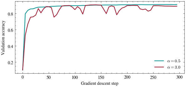
Change alpha_new below and re-run. Does a bigger step always get there sooner?

alpha_new = 3.0    # change me!

W2 = np.zeros((d, k))
val_accs2 = []
for t in range(n_steps):
    P_train = softmax(X_train @ W2)
    if t % 5 == 0:
        val_accs2.append(accuracy(softmax(X_val @ W2), y_val))
    W2 -= alpha_new * X_train.T @ (P_train - Y_train) / n_train

fig, ax = plt.subplots(figsize=(7, 3))
ax.plot(steps, val_accs, color=TEAL, linewidth=1.6, label=f"$\\alpha={alpha}$")
ax.plot(steps, val_accs2, color=CARDINAL, linewidth=1.6, label=f"$\\alpha={alpha_new}$")
ax.set_xlabel("Gradient descent step")
ax.set_ylabel("Validation accuracy")
ax.legend(frameon=False)
plt.show()

This linear softmax model reaches \(90.9\%\) accuracy on real handwritten digits using the softmax-minus-one-hot gradient derived in class. Its remaining errors reflect the linear decision boundary; the Neural Networks unit introduces nonlinear boundaries next.