Demo: Learned Decision Regions on a Spiral

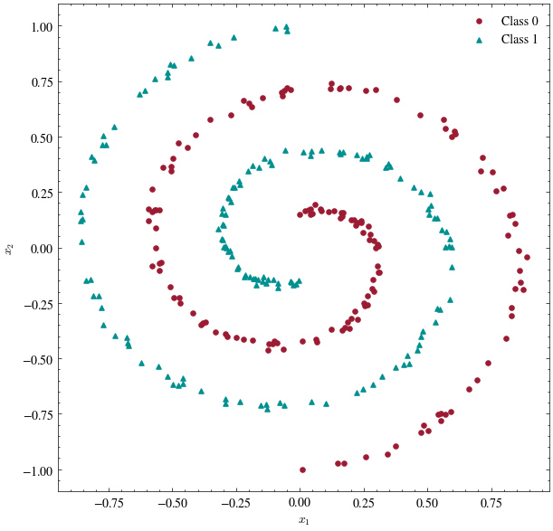
XOR was the smallest example that a linear model cannot separate. Here is a harder one: two interleaved spirals, with no straight line anywhere close to separating them. We train the network from the reading with our own forward and backward pass, then plot its decision region.

import numpy as np
import matplotlib.pyplot as plt
import scienceplots
from matplotlib.colors import LinearSegmentedColormap

plt.style.use(["science", "no-latex"])
TEAL, CARDINAL = "#009090", "#9c1b33"
FIELD = LinearSegmentedColormap.from_list("field", ["#ffffff", "#7a7a7a"])  # background shading
rng = np.random.default_rng(11)

n_per_class, noise = 150, 0.15
X, y = [], []
for c in [0, 1]:
    r = np.linspace(0.15, 1.0, n_per_class)
    t = np.linspace(c * np.pi, c * np.pi + 3.0 * np.pi, n_per_class) + rng.normal(0, noise, n_per_class)
    X.append(np.column_stack([r * np.sin(t), r * np.cos(t)]))
    y.append(np.full(n_per_class, c))
X, y = np.vstack(X), np.concatenate(y)

fig, ax = plt.subplots(figsize=(7, 7))
ax.scatter(*X[y == 0].T, color=CARDINAL, s=14, label="Class 0")
ax.scatter(*X[y == 1].T, color=TEAL, s=14, marker="^", label="Class 1")
ax.set_xlabel("$x_1$")
ax.set_ylabel("$x_2$")
ax.legend(frameon=False)
plt.show()

Before adding anything new, run last lecture’s model on it: one linear score per class, softmax on top, cross-entropy loss, trained with the softmax - one_hot gradient we derived at the board. How far does a straight boundary get?

def softmax(Z):
    Z = Z - Z.max(axis=1, keepdims=True)
    E = np.exp(Z)
    return E / E.sum(axis=1, keepdims=True)

Y = np.zeros((len(y), 2))          # one-hot labels
Y[np.arange(len(y)), y] = 1

rng_linear = np.random.default_rng(1)
W = rng_linear.normal(0, 0.1, size=(2, 2))
b = np.zeros(2)
for epoch in range(4000):
    P = softmax(X @ W + b)
    dZ = (P - Y) / len(X)
    W -= 1.0 * (X.T @ dZ)
    b -= 1.0 * dZ.sum(0)

linear_accuracy = np.mean(softmax(X @ W + b)[:, 1].round() == y)
print(f"linear model, training accuracy: {linear_accuracy:.1%}")

linear model, training accuracy: 66.3%

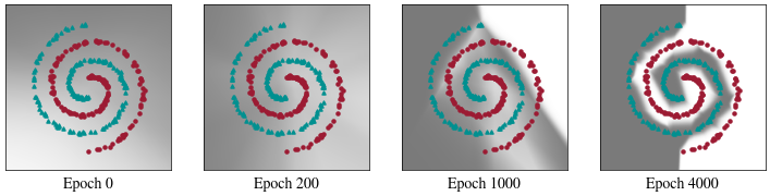
Now insert one hidden layer of ReLU neurons between the input and the logits. The backward pass is the reading’s, line for line: softmax minus one-hot at the top, an outer product for each weight gradient, and the ReLU mask on the way down.

def train(hidden_dim, n_epochs=4000, alpha=1.0, seed=1):
    n, d, k = len(X), 2, 2
    rng2 = np.random.default_rng(seed)
    W1 = rng2.normal(0, np.sqrt(2 / d), size=(d, hidden_dim)); b1 = np.zeros(hidden_dim)
    W2 = rng2.normal(0, np.sqrt(2 / hidden_dim), size=(hidden_dim, k)); b2 = np.zeros(k)
    snapshots = {}
    for epoch in range(n_epochs + 1):
        Z1 = X @ W1 + b1
        H = np.maximum(0, Z1)
        P = softmax(H @ W2 + b2)
        if epoch in (0, n_epochs // 20, n_epochs // 4, n_epochs):
            snapshots[epoch] = (W1.copy(), b1.copy(), W2.copy(), b2.copy())
        dZ2 = (P - Y) / n
        dZ1 = (dZ2 @ W2.T) * (Z1 > 0)
        W2 -= alpha * (H.T @ dZ2); b2 -= alpha * dZ2.sum(0)
        W1 -= alpha * (X.T @ dZ1); b1 -= alpha * dZ1.sum(0)
    return snapshots

def predict(params, points):
    W1, b1, W2, b2 = params
    H = np.maximum(0, points @ W1 + b1)
    return softmax(H @ W2 + b2)[:, 1]

snapshots = train(hidden_dim=64)
trained = snapshots[max(snapshots)]
print("snapshots at epochs:", list(snapshots))
print(f"64 hidden neurons, training accuracy: {np.mean(predict(trained, X).round() == y):.1%}")

snapshots at epochs: [0, 200, 1000, 4000]
64 hidden neurons, training accuracy: 100.0%

Plot the decision region at each snapshot: the background shading is the predicted probability of class \(1\), and the dots are the training data.

xx, yy = np.meshgrid(np.linspace(-1.3, 1.3, 200), np.linspace(-1.3, 1.3, 200))
grid = np.column_stack([xx.ravel(), yy.ravel()])

fig, axes = plt.subplots(1, 4, figsize=(9, 2.6))
for ax, epoch in zip(axes, snapshots):
    probs = predict(snapshots[epoch], grid).reshape(xx.shape)
    ax.imshow(probs, extent=[-1.3, 1.3, -1.3, 1.3], origin="lower", cmap=FIELD, vmin=0, vmax=1)
    ax.scatter(*X[y == 0].T, color=CARDINAL, s=5)
    ax.scatter(*X[y == 1].T, color=TEAL, s=5, marker="^")
    ax.set_xlabel(f"Epoch {epoch}")
    ax.set_xticks([]); ax.set_yticks([])
plt.show()

Reduce the hidden width

Sixty-four hidden neurons was generous. Try \(4\) below, barely more than XOR’s two, and compare the accuracy against the linear model’s.

hidden_dim = 4    # change me!

narrow = train(hidden_dim=hidden_dim)
params = narrow[max(narrow)]
probs = predict(params, grid).reshape(xx.shape)

fig, ax = plt.subplots(figsize=(7, 7))
ax.imshow(probs, extent=[-1.3, 1.3, -1.3, 1.3], origin="lower", cmap=FIELD, vmin=0, vmax=1)
ax.scatter(*X[y == 0].T, color=CARDINAL, s=10)
ax.scatter(*X[y == 1].T, color=TEAL, s=10, marker="^")
ax.set_xlabel(f"{hidden_dim} hidden neurons, epoch {max(narrow)}")
ax.set_xticks([]); ax.set_yticks([])
plt.show()

print(f"{hidden_dim} hidden neurons, training accuracy: {np.mean(predict(params, X).round() == y):.1%}")

4 hidden neurons, training accuracy: 66.0%

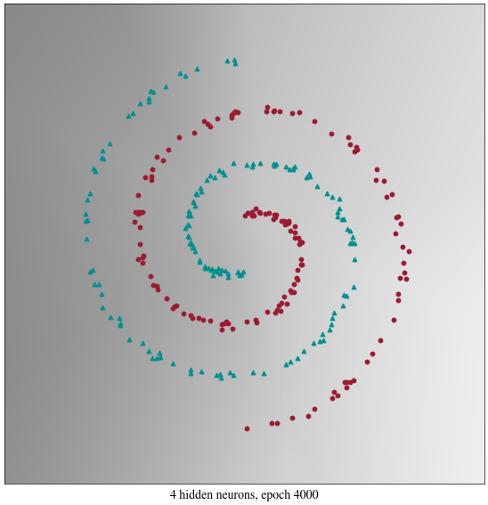
The network uses the same backpropagation equations as the small example in the reading, with larger matrices. Its \(322\) parameters reach \(100\%\) training accuracy on the spiral, compared with \(66\%\) for the linear model. With four hidden neurons, the network reaches the same accuracy as the linear model because it has too few creases to follow the spiral. Next lecture asks how to train a network like this one when the dataset is far too large to compute a full gradient over all of it at once.