Demo: Train a Neural Network on MNIST

We used MNIST to fit a linear classifier. Now we will learn a hidden layer as well, using PyTorch to compute gradients and Adam to update the weights.

This notebook uses torch, torchvision, and matplotlib. The first run downloads MNIST into data. Later runs reuse those files.

import matplotlib.pyplot as plt
import torch
from torch import nn
from torch.utils.data import DataLoader, random_split
from torchvision import datasets, transforms

plt.style.use("../figure_style.mplstyle")
torch.manual_seed(12)
device = torch.device("cuda" if torch.cuda.is_available() else "cpu")

Images and Batches

Each image has \(28\times28=784\) pixels, and its label is a digit from 0 to 9. ToTensor converts each image to a PyTorch tensor with pixel values in \([0,1]\).

MNIST provides 60,000 training images and a separate set of 10,000 test images. random_split divides the training set into 80% for training and 20% for validation. The test set stays separate until the final evaluation.

data = datasets.MNIST("data", train=True, download=True, transform=transforms.ToTensor())
training, validation = random_split(data, [0.8, 0.2])
test = datasets.MNIST("data", train=False, download=True, transform=transforms.ToTensor())

batch_size = 128
train_loader = DataLoader(training, batch_size=batch_size, shuffle=True)
train_eval_loader = DataLoader(training, batch_size=512)
validation_loader = DataLoader(validation, batch_size=512)
test_loader = DataLoader(test, batch_size=512)

fig, axes = plt.subplots(1, 8, figsize=(8, 1.5))
for ax, (image, label) in zip(axes, training):
    ax.imshow(image[0], cmap="gray_r", vmin=0, vmax=1)
    ax.set_title(str(label))
    ax.axis("off")
plt.show()

DataLoader shuffles the training examples and yields one batch at a time. One pass through train_loader is an epoch.

Network, Loss, and Optimizer

The network flattens each image, learns 128 ReLU features, and produces 10 class scores. nn.Linear includes trainable offsets by default, corresponding to the weights on constant features in the reading.

CrossEntropyLoss takes raw scores and integer labels. It includes the log-softmax calculation, so we do not put softmax at the end of the network. Adam receives the network’s parameters and a learning rate.

learning_rate = 0.001  # Change this, then rerun from this cell.
torch.manual_seed(12)
model = nn.Sequential(
    nn.Flatten(),
    nn.Linear(784, 128),
    nn.ReLU(),
    nn.Linear(128, 10),
).to(device)
loss_fn = nn.CrossEntropyLoss()
optimizer = torch.optim.Adam(model.parameters(), lr=learning_rate)

batch_images, batch_labels = next(iter(train_loader))
with torch.no_grad():
    scores = model(batch_images.to(device))
print(f"Images: {tuple(batch_images.shape)}")
print(f"Class scores: {tuple(scores.shape)}")
print(f"Labels: {tuple(batch_labels.shape)}")

Images: (128, 1, 28, 28)
Class scores: (128, 10)
Labels: (128,)

The first dimension counts examples in the batch. Each row of scores contains ten logits for one image.

Before training, what accuracy would you expect on ten digit classes? The following function measures loss and accuracy without changing the weights. model.eval() selects evaluation behavior, and torch.no_grad() avoids storing computations for a backward pass.

def evaluate(loader):
    model.eval()
    total_loss, correct, count = 0.0, 0, 0
    with torch.no_grad():
        for batch_images, batch_labels in loader:
            batch_images = batch_images.to(device)
            batch_labels = batch_labels.to(device)
            scores = model(batch_images)
            total_loss += loss_fn(scores, batch_labels).item() * len(batch_labels)
            correct += (scores.argmax(dim=1) == batch_labels).sum().item()
            count += len(batch_labels)
    return total_loss / count, correct / count

initial_loss, initial_accuracy = evaluate(validation_loader)
print(f"Before training: loss {initial_loss:.3f}, accuracy {initial_accuracy:.1%}")

Before training: loss 2.297, accuracy 12.3%

Train

Each batch follows the same sequence: clear the old gradients, compute the scores and loss, run the backward pass, and update the parameters. PyTorch accumulates gradients, which is why we call zero_grad() before each backward pass.

Predict how training and validation loss will change over five epochs.

epochs = 5
train_loss, train_accuracy = evaluate(train_eval_loader)
history = {
    "train_loss": [train_loss],
    "validation_loss": [initial_loss],
    "train_accuracy": [train_accuracy],
    "validation_accuracy": [initial_accuracy],
}

for epoch in range(epochs):
    model.train()
    for batch_images, batch_labels in train_loader:
        batch_images = batch_images.to(device)
        batch_labels = batch_labels.to(device)

        optimizer.zero_grad()
        scores = model(batch_images)
        loss = loss_fn(scores, batch_labels)
        loss.backward()
        optimizer.step()

    train_loss, train_accuracy = evaluate(train_eval_loader)
    validation_loss, validation_accuracy = evaluate(validation_loader)
    history["train_loss"].append(train_loss)
    history["validation_loss"].append(validation_loss)
    history["train_accuracy"].append(train_accuracy)
    history["validation_accuracy"].append(validation_accuracy)

print(f"After {epochs} epochs: training accuracy {train_accuracy:.1%}, "
      f"validation accuracy {validation_accuracy:.1%}")

After 5 epochs: training accuracy 97.7%, validation accuracy 96.7%

Both curves below evaluate the current weights on a fixed dataset after each epoch. Validation images contribute no training gradients.

plt.plot(history["train_loss"], label="Training")
plt.plot(history["validation_loss"], label="Validation")
plt.xlabel("Epoch")
plt.ylabel("Cross-Entropy")
plt.legend()
plt.show()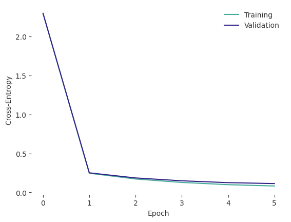

Test on New Digits

We now evaluate the trained network on the untouched test set. A predicted label is the index of the largest logit. Softmax would give the same predicted class.

test_loss, test_accuracy = evaluate(test_loader)
print(f"Test loss: {test_loss:.3f}")
print(f"Test accuracy: {test_accuracy:.1%}")

model.eval()
with torch.no_grad():
    predictions = torch.cat([
        model(images.to(device)).argmax(dim=1).cpu()
        for images, labels in test_loader
    ])

mistakes = torch.where(predictions != test.targets)[0][:8]
fig, axes = plt.subplots(1, 8, figsize=(8, 1.8))
for ax in axes:
    ax.axis("off")
for ax, index in zip(axes, mistakes):
    image, label = test[int(index)]
    ax.imshow(image[0], cmap="gray_r", vmin=0, vmax=1)
    ax.set_title(f"{label} → {predictions[index].item()}")
fig.suptitle("Test Mistakes: Label → Prediction")
plt.show()

Test loss: 0.104
Test accuracy: 96.9%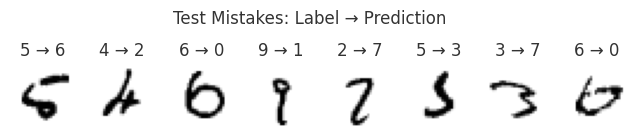

What do the mistakes have in common? Change learning_rate and rerun from the model cell to compare the validation curves from the same initialization. Use validation performance to choose the rate.

For more on the training loop, see the PyTorch quickstart.