We run one forward and backward pass through a \(30\)-layer network, deep enough to measure the exponential behavior in the reading’s bound. At every layer we track the activation standard deviation in the forward pass and the gradient norm in the backward pass. torch.autograd computes the gradients.
import numpy as npimport matplotlib.pyplot as pltimport scienceplotsimport torchplt.style.use(["science", "no-latex"])TEAL, CARDINAL, GRAY ="#009090", "#9c1b33", "#c9c9c9"torch.manual_seed(13)width, depth =128, 30def make_layers(depth, width, std): layers = []for _ inrange(depth): lin = torch.nn.Linear(width, width, bias=False)with torch.no_grad(): lin.weight.normal_(0, std) layers.append(lin)return layersdef run_plain(layers, x, activation): h = x acts = []for lin in layers: h = activation(lin(h)) h.retain_grad() acts.append(h) loss = h.pow(2).sum() loss.backward() act_stds = [a.detach().std().item() for a in acts] grad_norms = [a.grad.norm().item() for a in acts]return act_stds, grad_normsx = torch.randn(256, width)configs = [ ("Too small ($0.5/\\sqrt{n_{\\mathrm{in}}}$)", 0.5/ width **0.5, CARDINAL), ("Well-scaled ($1/\\sqrt{n_{\\mathrm{in}}}$)", 1.0/ width **0.5, TEAL), ("Too large ($3/\\sqrt{n_{\\mathrm{in}}}$)", 3.0/ width **0.5, "black"),]fig, axes = plt.subplots(1, 2, figsize=(9, 3.2))layer_idx = np.arange(1, depth +1)for label, std, color in configs: layers = make_layers(depth, width, std) act_stds, grad_norms = run_plain(layers, x.clone(), torch.tanh) axes[0].plot(layer_idx, act_stds, color=color, linewidth=1.5, label=label) axes[1].plot(layer_idx, grad_norms, color=color, linewidth=1.5, label=label) rho = (grad_norms[0] / grad_norms[-1]) ** (1/ (depth -1))print(f"std {std:.4f}: act std {act_stds[0]:8.3g} -> {act_stds[-1]:8.3g} | "f"grad {grad_norms[-1]:8.3g} (output) -> {grad_norms[0]:8.3g} (input) | rho = {rho:.2f}")axes[0].set_yscale("log"); axes[0].set_xlabel("Layer"); axes[0].set_ylabel("Activation std (log scale)")axes[1].set_yscale("log"); axes[1].set_xlabel("Layer"); axes[1].set_ylabel("Gradient norm (log scale)")axes[1].legend(frameon=False, fontsize=7, loc="lower right")plt.show()
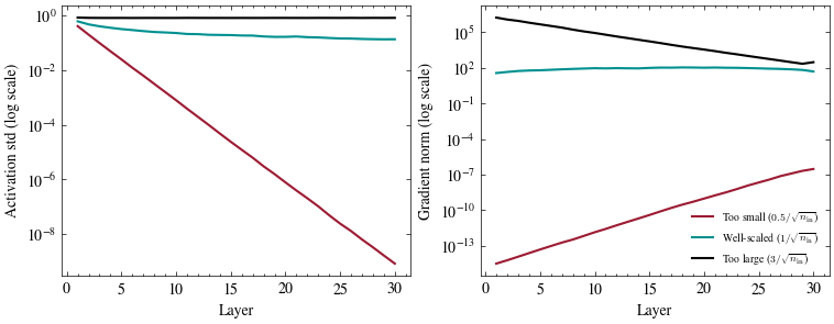
Three initialization scales, same depth, same input. On the left the forward signal: the too-small network’s activation standard deviation falls from \(0.42\) to \(8\times10^{-10}\), while the too-large one holds near \(0.85\) only because its \(\tanh\) units are saturated. On the right the gradient, running the other way: the too-small network’s falls from \(3\times 10^{-7}\) at the output to \(3\times 10^{-15}\) at the input, and the too-large network’s grows from \(3\times 10^{2}\) to \(2\times 10^{6}\) going the same direction. Each gradient curve is a straight line on the log axis, and its slope is the per-layer factor \(\rho\) from the reading’s bound: \(0.53\), \(0.99\), and \(1.35\).
Compare residual connections and layer normalization
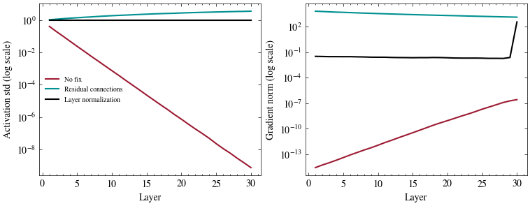
Take the worst case above (too-small init) and compare three versions: no fix, residual connections, and layer normalization.
std_small =0.5/ width **0.5def run_residual(layers, x, activation): h = x acts = []for lin in layers: h = h + activation(lin(h)) h.retain_grad() acts.append(h) loss = h.pow(2).sum() loss.backward()return [a.detach().std().item() for a in acts], [a.grad.norm().item() for a in acts]def run_layernorm(layers, x, activation): ln = torch.nn.LayerNorm(width) h = x acts = []for lin in layers: h = ln(activation(lin(h))) h.retain_grad() acts.append(h) loss = h.pow(2).sum() loss.backward()return [a.detach().std().item() for a in acts], [a.grad.norm().item() for a in acts]torch.manual_seed(13)act_plain, grad_plain = run_plain(make_layers(depth, width, std_small), x.clone(), torch.tanh)torch.manual_seed(13)act_residual, grad_residual = run_residual(make_layers(depth, width, std_small), x.clone(), torch.tanh)torch.manual_seed(13)act_layernorm, grad_layernorm = run_layernorm(make_layers(depth, width, std_small), x.clone(), torch.tanh)runs = [ ("No fix", act_plain, grad_plain, CARDINAL), ("Residual connections", act_residual, grad_residual, TEAL), ("Layer normalization", act_layernorm, grad_layernorm, "black"),]fig, axes = plt.subplots(1, 2, figsize=(9, 3.2))layer_idx = np.arange(1, depth +1)for label, acts, grads, color in runs: axes[0].plot(layer_idx, acts, color=color, linewidth=1.5, label=label) axes[1].plot(layer_idx, grads, color=color, linewidth=1.5, label=label)axes[0].set_yscale("log"); axes[0].set_xlabel("Layer"); axes[0].set_ylabel("Activation std (log scale)")axes[0].legend(frameon=False, fontsize=7, loc="center left")axes[1].set_yscale("log"); axes[1].set_xlabel("Layer"); axes[1].set_ylabel("Gradient norm (log scale)")plt.show()for label, acts, grads, _ in runs:print(f"{label:22s} act std {acts[0]:8.3g} -> {acts[-1]:8.3g} | "f"grad {grads[-1]:8.3g} (output) -> {grads[0]:8.3g} (input)")
Both changes prevent the gradient from decaying in the same badly initialized network, but their forward scales differ. The residual stream (teal) lets the forward signal grow, from \(1.1\) to \(3.7\), because every block adds onto it; layer normalization (black) keeps it at exactly \(1\) at every layer. On the gradient side, residual connections keep the absolute size between \(1\times 10^{3}\) and \(7\times 10^{3}\) because each block includes an identity path. Layer norm drops once at the output, where the loss is applied, and then holds a small but steady scale between \(1.9\times 10^{-2}\) and \(3.3\times 10^{-2}\) for every remaining layer. Different scales, same property: neither gradient curve decays with depth.
Increase the depth to 100 layers
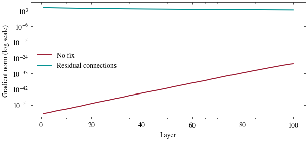
Try depth = 100 below and re-run to see how much worse the unfixed network gets, and whether the fix still holds up. At that depth the unfixed network’s loss underflows to zero in single precision, so the cell uses double precision.
depth_new =100# change me!# Double precision, because at depth 100 the unfixed loss underflows float32 to exactly 0.x2 = torch.randn(256, width).double()torch.manual_seed(13)_, g_plain = run_plain([l.double() for l in make_layers(depth_new, width, std_small)], x2.clone(), torch.tanh)torch.manual_seed(13)_, g_res = run_residual([l.double() for l in make_layers(depth_new, width, std_small)], x2.clone(), torch.tanh)fig, ax = plt.subplots(figsize=(7, 3))layer_idx = np.arange(1, depth_new +1)ax.plot(layer_idx, g_plain, color=CARDINAL, linewidth=1.4, label="No fix")ax.plot(layer_idx, g_res, color=TEAL, linewidth=1.4, label="Residual connections")ax.set_yscale("log")ax.set_xlabel("Layer")ax.set_ylabel("Gradient norm (log scale)")ax.legend(frameon=False, loc="center left")plt.show()
Each extra layer multiplies the unfixed network’s gradient by a factor below \(1\), producing the exponential decay predicted by the reading’s spectral-norm bound. In this experiment, the residual network’s identity paths keep the gradient from decaying through 100 layers.