Demo: Low-rank Approximation of an Image and a Video

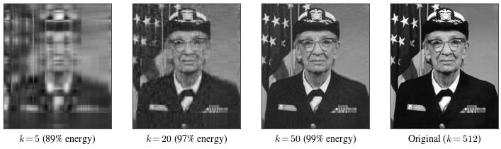
We use the photograph from the Linear Algebra warp demo and truncate its SVD at several ranks. Then we do the same thing to a video.

import numpy as np
import matplotlib.pyplot as plt
import matplotlib.cbook as cbook
import scienceplots

plt.style.use(["science", "no-latex"])
TEAL, CARDINAL, GRAY = "#009090", "#9c1b33", "#c9c9c9"

with cbook.get_sample_data("grace_hopper.jpg") as f:
    img = plt.imread(f)
gray = img.mean(axis=2)
u, s, vt = np.linalg.svd(gray, full_matrices=False)
print(f"image shape: {gray.shape}, {len(s)} singular values")

image shape: (600, 512), 512 singular values

def rank_k(u, s, vt, k):
    return (u[:, :k] * s[:k]) @ vt[:k, :]

total_energy = np.sum(s ** 2)
fig, axes = plt.subplots(1, 4, figsize=(9, 3))
for ax, k in zip(axes[:3], [5, 20, 50]):
    approx = rank_k(u, s, vt, k)
    captured = np.sum(s[:k] ** 2) / total_energy
    ax.imshow(approx, cmap="gray")
    ax.set_xlabel(f"$k={k}$ ({captured:.0%} energy)")
    ax.set_xticks([]); ax.set_yticks([])
axes[3].imshow(gray, cmap="gray")
axes[3].set_xlabel(f"Original ($k={len(s)}$)")
axes[3].set_xticks([]); axes[3].set_yticks([])
plt.show()

Inspect the singular-value spectrum

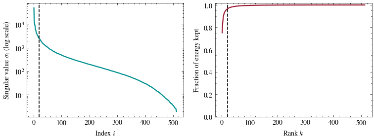
The reason \(k=20\) gets that close is the shape of the spectrum. On the left, the singular values on a log scale; on the right, the fraction of the energy \(\sum_i \sigma_i^2\) kept by a rank-\(k\) truncation. The dashed line marks \(k=20\) in both.

idx = np.arange(1, len(s) + 1)
cumulative = np.cumsum(s ** 2) / total_energy
n, d = gray.shape

fig, axes = plt.subplots(1, 2, figsize=(9, 3))
axes[0].plot(idx, s, color=TEAL, linewidth=1.6)
axes[0].axvline(20, color="black", linestyle="--", linewidth=1.2)
axes[0].set_yscale("log")
axes[0].set_xlabel("Index $i$")
axes[0].set_ylabel("Singular value $\\sigma_i$ (log scale)")

axes[1].plot(idx, cumulative, color=CARDINAL, linewidth=1.6)
axes[1].axvline(20, color="black", linestyle="--", linewidth=1.2)
axes[1].set_ylim(0, 1.02)
axes[1].set_xlabel("Rank $k$")
axes[1].set_ylabel("Fraction of energy kept")
plt.show()

print(f"rank 20 keeps {cumulative[19]:.0%} of the energy")
print(f"rank 20 costs {20 * (n + d + 1) / (n * d):.0%} of the storage")

rank 20 keeps 97% of the energy
rank 20 costs 7% of the storage

Apply the same method to video

Flatten every frame of a short video into one column of a matrix (pixels \(\times\) frames). Its singular values measure how many directions contain most of the video’s energy.

rng = np.random.default_rng(15)
T, H, W = 60, 40, 40
xs, ys = np.meshgrid(np.arange(W), np.arange(H))

frames = []
for t in range(T):
    cx = 5 + (W - 10) * t / (T - 1)   # a blob drifting left to right
    cy = H / 2
    frame = np.exp(-((xs - cx) ** 2 + (ys - cy) ** 2) / (2 * 6 ** 2))
    frame += rng.normal(0, 0.02, size=frame.shape)
    frames.append(frame.ravel())

M = np.array(frames).T   # (H*W) x T: one column per frame
print("video-as-matrix shape:", M.shape)

u_v, s_v, vt_v = np.linalg.svd(M, full_matrices=False)
total_v = np.sum(s_v ** 2)
for k in [1, 2, 3, 5]:
    print(f"rank {k}: {np.sum(s_v[:k] ** 2) / total_v:.1%} of the video's energy")

video-as-matrix shape: (1600, 60)
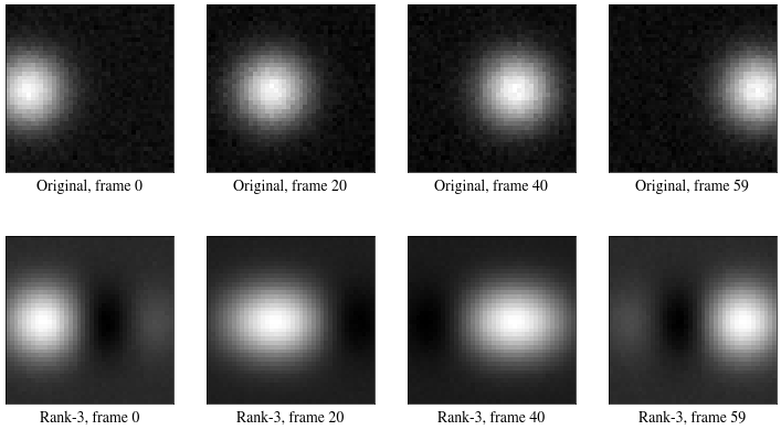
rank 1: 56.7% of the video's energy
rank 2: 86.2% of the video's energy
rank 3: 96.5% of the video's energy
rank 5: 99.4% of the video's energy

fig, axes = plt.subplots(2, 4, figsize=(9, 5))
frame_ids = [0, 20, 40, 59]
for col, t in enumerate(frame_ids):
    axes[0, col].imshow(frames[t].reshape(H, W), cmap="gray")
    axes[0, col].set_xlabel(f"Original, frame {t}")
    axes[0, col].set_xticks([]); axes[0, col].set_yticks([])

k = 3
M_k = rank_k(u_v, s_v, vt_v, k)
for col, t in enumerate(frame_ids):
    axes[1, col].imshow(M_k[:, t].reshape(H, W), cmap="gray")
    axes[1, col].set_xlabel(f"Rank-{k}, frame {t}")
    axes[1, col].set_xticks([]); axes[1, col].set_yticks([])
plt.show()

For this moving-blob video, rank \(3\) retains nearly all of the visible motion.

Add more noise

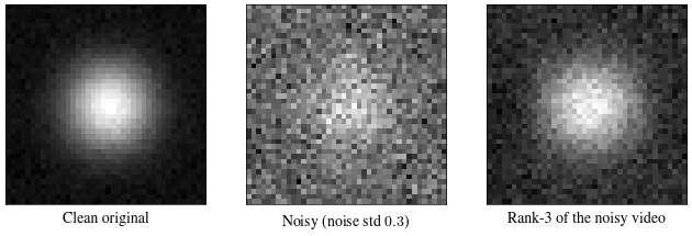
When the signal is concentrated in a few singular directions, low-rank reconstruction should discard more noise than signal. Try noise_std = 0.3 below (much noisier than the 0.02 used above) and compare the rank-\(3\) reconstruction with the noisy original.

noise_std = 0.3    # change me!

frames_noisy = []
for t in range(T):
    cx = 5 + (W - 10) * t / (T - 1)
    cy = H / 2
    frame = np.exp(-((xs - cx) ** 2 + (ys - cy) ** 2) / (2 * 6 ** 2))
    frame += rng.normal(0, noise_std, size=frame.shape)
    frames_noisy.append(frame.ravel())

M_noisy = np.array(frames_noisy).T
u_n, s_n, vt_n = np.linalg.svd(M_noisy, full_matrices=False)
M_noisy_k = rank_k(u_n, s_n, vt_n, 3)

fig, axes = plt.subplots(1, 3, figsize=(8, 3))
t_show = 30
axes[0].imshow(frames[t_show].reshape(H, W), cmap="gray")
axes[0].set_xlabel("Clean original")
axes[1].imshow(frames_noisy[t_show].reshape(H, W), cmap="gray")
axes[1].set_xlabel(f"Noisy (noise std ${noise_std}$)")
axes[2].imshow(M_noisy_k[:, t_show].reshape(H, W), cmap="gray")
axes[2].set_xlabel("Rank-3 of the noisy video")
for ax in axes:
    ax.set_xticks([]); ax.set_yticks([])
plt.show()

The rank-\(3\) reconstruction of the noisy video is close to the clean original. The blob’s motion is concentrated in the top three singular directions, while the noise is spread across all \(60\), so truncation removes more noise than signal.