Embeddings

Last lecture proved that truncating the SVD gives the best rank-\(k\) approximation of a matrix, and we spent the hour approximating an image. Today we apply the same theorem to a data matrix, with one row per data point. A rank-\(k\) approximation gives a compressed description of every row. That compressed description is an embedding. A language model receives a token’s embedding rather than its discrete vocabulary index. We will find the reconstruction-optimal linear compression to \(k\) numbers and determine which properties of those coordinates are identifiable.

Dense Representations

An embedding of a data point \(\mathbf{x}\) is a short list of numbers standing in for it: \[ \mathbf{z} = \phi(\mathbf{x}) \in \mathbb{R}^k, \] where \(\phi\) is a map we either choose or learn and \(k\) is the embedding dimension, usually a few dozen to a few thousand. The word dense means that essentially every coordinate of \(\mathbf{z}\) is nonzero and carries information.

The contrast is a sparse representation, and the standard example is the one-hot vector. Give a vocabulary of \(|V|\) words an arbitrary ordering and represent word \(i\) by \(\mathbf{e}_i\in\mathbb{R}^{|V|}\), all zeros except a single \(1\) in position \(i\). A real vocabulary can exceed a hundred thousand words, so each one-hot vector has that many coordinates. It also places every pair of distinct words at the same distance: \[ \|\mathbf{e}_i - \mathbf{e}_j\|^2 = \|\mathbf{e}_i\|^2 - 2\langle \mathbf{e}_i,\mathbf{e}_j\rangle + \|\mathbf{e}_j\|^2 = 1 - 0 + 1 = 2 . \] Thus “cat” is as far from “dog” as it is from “molybdenum.” A useful dense embedding in \(\mathbb{R}^{50}\) can instead place related words nearby.

We first find the linear map \(\phi\) with the smallest reconstruction error.

The Linear Autoencoder

Take the dataset to be a matrix \(\mathbf{X}\in\mathbb{R}^{n\times d}\) of \(n\) points with \(d\) features each, whose \(i\)th row is \((\mathbf{x}^{(i)})^\top\), and fix a budget \(k < d\). The simplest map we can write down is a linear one. An encoder matrix \(\mathbf{W}_0\in\mathbb{R}^{d\times k}\) compresses a point to its code: \[ \mathbf{z} = \mathbf{W}_0^\top\mathbf{x} \in\mathbb{R}^k . \] A decoder matrix \(\mathbf{W}_1\in\mathbb{R}^{k\times d}\) expands the code back into the original space: \[ \hat{\mathbf{x}} = \mathbf{W}_1^\top\mathbf{z} \in\mathbb{R}^d . \] The pair \((\mathbf{W}_0,\mathbf{W}_1)\) is a linear autoencoder, trained to minimize the error after this round trip. Stacking the reconstructions into a matrix \(\hat{\mathbf{X}}\in\mathbb{R}^{n\times d}\) whose \(i\)th row is \((\hat{\mathbf{x}}^{(i)})^\top\), the loss is the total squared reconstruction error: \[ \mathcal{L}(\mathbf{W}_0,\mathbf{W}_1) = \|\mathbf{X}-\hat{\mathbf{X}}\|_F^2, \qquad \hat{\mathbf{X}} = \mathbf{X}\mathbf{W}_0\mathbf{W}_1 . \]

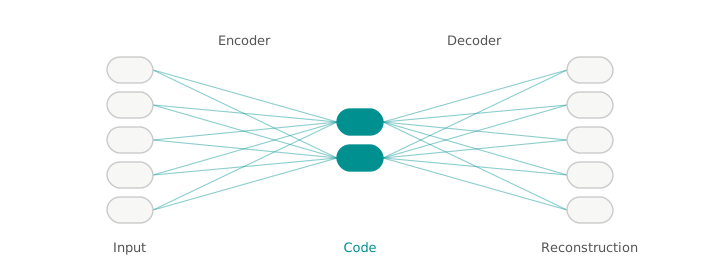
In the diagram, the input coordinates pass through the smaller set of code coordinates before being expanded back to the original dimension. Every reconstruction factors as \(\hat{\mathbf{X}} = (\mathbf{X}\mathbf{W}_0)\mathbf{W}_1\) through the \(n\times k\) matrix \(\mathbf{X}\mathbf{W}_0\), and the rank of a product is at most the smallest dimension it passes through, so: \[ \mathrm{rank}(\hat{\mathbf{X}}) \leq k . \] Training a linear autoencoder therefore searches within the rank-\(\leq k\) matrices from last lecture. The Eckart–Young–Mirsky theorem gives the optimal reconstruction directly.

Principal Component Analysis

Every rank-\(k\) matrix has rows in a \(k\)-dimensional subspace through the origin. If the data cloud is far from the origin, a rank-\(1\) approximation may use its single direction largely to represent the mean rather than variation around it. The fix is to move the origin to the data, defining the mean row and the centered data matrix: \[ \bar{\mathbf{x}} = \frac1n\sum_{i=1}^n \mathbf{x}^{(i)} \in\mathbb{R}^d, \qquad \mathbf{X}_c = \mathbf{X} - \mathbf{1}\bar{\mathbf{x}}^\top \in\mathbb{R}^{n\times d}, \] where \(\mathbf{1}\in\mathbb{R}^n\) is the all-ones vector, so every column of \(\mathbf{X}_c\) now sums to zero. Write the SVD of the centered matrix in the outer-product form from the Decompositions lecture: \[ \mathbf{X}_c = \sum_{i=1}^r \sigma_i\mathbf{u}_i\mathbf{v}_i^\top, \qquad \sigma_1\geq\sigma_2\geq\cdots\geq\sigma_r>0 . \] The top \(k\) right singular vectors \(\mathbf{v}_1,\ldots,\mathbf{v}_k\in\mathbb{R}^d\) are the principal components, collected as the columns of one matrix: \[ \mathbf{V}_k = [\,\mathbf{v}_1\ \cdots\ \mathbf{v}_k\,] \in\mathbb{R}^{d\times k} . \] Principal component analysis (PCA) is the embedding that centers, then projects onto those \(k\) directions: \[ \mathbf{z} = \mathbf{V}_k^\top(\mathbf{x}-\bar{\mathbf{x}}), \qquad \hat{\mathbf{x}} = \bar{\mathbf{x}} + \mathbf{V}_k\mathbf{z} . \] PCA is written as a projection rather than as a pair of trained matrices, but the claim below bounds the error of any rank-\(k\) reconstruction, so it covers every linear autoencoder at once.

Claim: Let \(\hat{\mathbf{X}} = \mathbf{1}\bar{\mathbf{x}}^\top + \mathbf{B}\) be any reconstruction built from an offset plus a matrix \(\mathbf{B}\) of rank at most \(k\). Its squared error is at least the tail energy: \[ \|\mathbf{X}-\hat{\mathbf{X}}\|_F^2 \;\geq\; \sum_{i=k+1}^r \sigma_i^2, \] with equality for PCA’s choice \(\mathbf{B} = \mathbf{X}_c\mathbf{V}_k\mathbf{V}_k^\top\).

Proof of Claim

Subtracting the offset turns the error into an error on the centered matrix, since \(\mathbf{X}-\mathbf{1}\bar{\mathbf{x}}^\top = \mathbf{X}_c\): \[ \|\mathbf{X}-\hat{\mathbf{X}}\|_F^2 = \|\mathbf{X} - \mathbf{1}\bar{\mathbf{x}}^\top - \mathbf{B}\|_F^2 = \|\mathbf{X}_c-\mathbf{B}\|_F^2 . \] Now \(\mathbf{B}\) ranges over all matrices of rank at most \(k\), so last lecture’s theorem applies verbatim: the minimum of \(\|\mathbf{X}_c-\mathbf{B}\|_F^2\) is the tail energy \(\sum_{i>k}\sigma_i^2\), attained by the truncated SVD \((\mathbf{X}_c)_k = \sum_{i=1}^k\sigma_i\mathbf{u}_i\mathbf{v}_i^\top\).

It remains to check that PCA’s choice is that truncated SVD. Substitute the SVD and expand \(\mathbf{V}_k\mathbf{V}_k^\top = \sum_{j=1}^k \mathbf{v}_j\mathbf{v}_j^\top\): \[ \begin{align*} \mathbf{X}_c\mathbf{V}_k\mathbf{V}_k^\top &= \Big(\sum_{i=1}^r \sigma_i\mathbf{u}_i\mathbf{v}_i^\top\Big)\Big(\sum_{j=1}^k \mathbf{v}_j\mathbf{v}_j^\top\Big) \\&= \sum_{i=1}^r\sum_{j=1}^k \sigma_i\,\mathbf{u}_i\,(\mathbf{v}_i^\top\mathbf{v}_j)\,\mathbf{v}_j^\top \\&= \sum_{i=1}^k \sigma_i\mathbf{u}_i\mathbf{v}_i^\top \;=\; (\mathbf{X}_c)_k , \end{align*} \] where orthonormality of the right singular vectors (\(\mathbf{v}_i^\top\mathbf{v}_j = 0\) unless \(i = j\)) kills every cross term, leaving only the indices \(i\leq k\).

The error \(\sum_{i>k}\sigma_i^2\) is exactly last lecture’s tail energy, and dividing by the total energy gives the share of the data’s spread that a \(k\)-dimensional embedding keeps: \[ \frac{\sigma_1^2+\cdots+\sigma_k^2}{\sigma_1^2+\cdots+\sigma_r^2} . \] This quantity is the “variance explained” by the top \(k\) components. Among all unit directions, the variance of the centered points is largest along \(\mathbf{v}_1\), so the principal components are the directions of greatest spread. The matrix \(\frac1n\mathbf{X}_c^\top\mathbf{X}_c\) whose eigenvectors they are is the data’s covariance matrix.

The objective uses only squared distance, not downstream utility. PCA can therefore discard a low-variance feature even if it separates two classes perfectly. If the data already lies in a \(k\)-dimensional subspace, every singular value after the first \(k\) is zero, so the reconstruction error is zero.

One Principal Component by Hand

Take four points in the plane, \((5,6)\), \((1,2)\), \((4,3)\), and \((2,5)\), and compress each of them to \(k=1\) number.

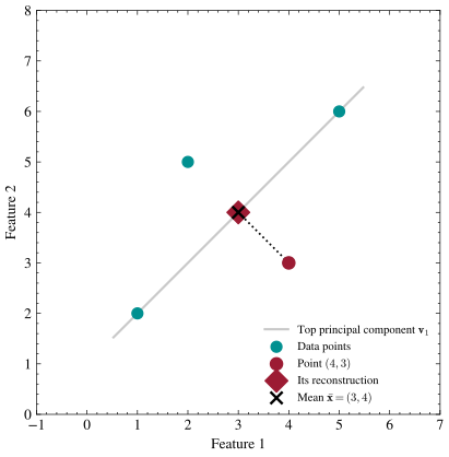
Their mean is \(\bar{\mathbf{x}} = (3,4)\), marked in the plot with a black cross, so centering gives the four points \((2,2)\), \((-2,-2)\), \((1,-1)\), and \((-1,1)\). Summing outer products gives the matrix whose eigenvectors we want: \[ \mathbf{X}_c^\top\mathbf{X}_c = \sum_{i=1}^4 \mathbf{x}_c^{(i)}(\mathbf{x}_c^{(i)})^\top = \begin{bmatrix}10 & 6\\ 6 & 10\end{bmatrix} . \] A symmetric matrix of the form \(\begin{bmatrix}a & b\\ b& a\end{bmatrix}\) always has eigenvectors \((1,1)/\sqrt2\) and \((1,-1)/\sqrt2\), with eigenvalues \(a+b\) and \(a-b\), so here \(\sigma_1^2 = 16\) and \(\sigma_2^2 = 4\). The top principal component is therefore \(\mathbf{v}_1 = (1,1)/\sqrt{2}\), the \(45°\) line drawn in gray through the mean, and keeping one component keeps \(16/20 = 80\%\) of the spread.

Now compress the point \((4,3)\), drawn in cardinal red. Centered it is \((1,-1)\), and its single code number is its coordinate along \(\mathbf{v}_1\): \[ z = \mathbf{v}_1^\top(\mathbf{x}-\bar{\mathbf{x}}) = \frac{1}{\sqrt2}\big((1)(1) + (1)(-1)\big) = 0 . \] Its deviation from the mean is entirely perpendicular to the direction we kept, so its reconstruction is the mean itself, \(\hat{\mathbf{x}} = \bar{\mathbf{x}} + 0\cdot\mathbf{v}_1 = (3,4)\), the cardinal diamond drawn at the black cross. Its reconstruction error is the length of the dotted segment: \[ \|\mathbf{x}-\hat{\mathbf{x}}\| = \|(4,3)-(3,4)\| = \sqrt{1+1} = \sqrt{2} \approx 1.41 . \] In the plot, \((4,3)\) and \((2,5)\) sit off the gray line and tie for the worst error, while \((5,6)\) and \((1,2)\) lie exactly on it and are reconstructed perfectly.

Summing the four squared errors gives \(0 + 0 + 2 + 2 = 4\), exactly the tail energy \(\sigma_2^2 = 4\) the claim predicted, with no slack in the bound.

PCA is optimal, but only among linear maps \(\phi\) and only for the reconstruction loss, and lifting those two restrictions is what the rest of representation learning is about.

Learning Embeddings by Self-Supervision

Replacing \(\mathbf{W}_0\) and \(\mathbf{W}_1\) with neural networks allows nonlinear embeddings. Self-supervised learning derives training targets from the data itself, so a model can train on unannotated text or images. Common objectives include reconstruction, autoregressive prediction, and contrastive learning.

Reconstruction is the autoencoder above with the linearity dropped. Let \(\phi:\mathbb{R}^d\to\mathbb{R}^k\) and \(\psi:\mathbb{R}^k\to\mathbb{R}^d\) be networks standing in for \(\mathbf{W}_0^\top\) and \(\mathbf{W}_1^\top\), and train them on the same objective: \[ \mathcal{L} = \sum_{i=1}^n \big\|\mathbf{x}^{(i)} - \psi\big(\phi(\mathbf{x}^{(i)})\big)\big\|^2 . \] Because a nonlinear \(\phi\) can bend the data before projecting it, the embedding can capture curved structure that no choice of \(\mathbf{V}_k\) ever could.

Autoregressive prediction predicts future tokens from earlier ones. Given a sequence \(x_1,\ldots,x_T\) of tokens, predict each one from everything before it, which is maximum likelihood on the sequence: \[ \mathcal{L} = -\sum_{t=1}^{T} \log \Pr(x_t \mid x_1,\ldots,x_{t-1}) . \] This is the cross-entropy loss from the Logistic Regression lecture, with a softmax over the whole vocabulary supplying the probabilities. The internal vector used to predict the next token serves as an embedding of the preceding sequence. The Architectures unit builds the transformer around this objective.

Contrastive learning uses pairs known to belong together, such as two crops of one photograph, and pairs that do not, such as two random photographs. Given an anchor \(\mathbf{z}\), a positive partner \(\mathbf{z}^+\), and \(m\) negatives \(\mathbf{z}^-_1,\ldots,\mathbf{z}^-_m\), the loss classifies the positive partner among \(m+1\) candidates: \[ \mathcal{L} = -\log \frac{\exp\big(\langle\mathbf{z},\mathbf{z}^+\rangle/\tau\big)}{\exp\big(\langle\mathbf{z},\mathbf{z}^+\rangle/\tau\big) + \sum_{j=1}^m \exp\big(\langle\mathbf{z},\mathbf{z}^-_j\rangle/\tau\big)}, \] where \(\tau>0\) is a temperature controlling how sharply the softmax discriminates. That fraction is a softmax over \(m+1\) candidates and the loss is its cross-entropy again: a classification problem whose classes are “which of these is my partner.”

These losses do not assign a fixed meaning to each coordinate of \(\mathbf{z}\). They constrain relative positions, which motivates comparing distances and directions in the embedding space.

The Geometry of Embedding Space

Two embeddings are compared in one of two ways: Euclidean distance \(\|\mathbf{z}_1-\mathbf{z}_2\|\), or cosine similarity, the cosine of the angle between them: \[ \cos(\mathbf{z}_1,\mathbf{z}_2) = \frac{\langle\mathbf{z}_1,\mathbf{z}_2\rangle}{\|\mathbf{z}_1\|\,\|\mathbf{z}_2\|} \in [-1,1] . \] Cosine similarity keeps only direction, usually the right trade for words: a vector’s length tracks how often a word appears more than what it means. For unit-length embeddings, the squared Euclidean distance is determined by cosine similarity: \[ \|\mathbf{z}_1-\mathbf{z}_2\|^2 = \|\mathbf{z}_1\|^2 - 2\langle\mathbf{z}_1,\mathbf{z}_2\rangle + \|\mathbf{z}_2\|^2 = 2 - 2\cos(\mathbf{z}_1,\mathbf{z}_2) . \] On the unit sphere, “closest” and “most similar” produce the same list; the two measures can only disagree when lengths differ.

Given a query embedding \(\mathbf{z}\) and \(N\) stored embeddings, its nearest neighbors are the stored vectors with the largest similarity to it. Brute-force search uses one inner product per stored vector, or \(O(Nk)\) time per query.

GloVe trains embeddings by minimizing a weighted least-squares objective on log co-occurrence counts from a large text corpus. Its training targets come from the corpus, but its objective is a matrix-factorization loss rather than the autoregressive objective above. The resulting vectors place many related words near one another in \(\mathbb{R}^{50}\). Some relations also appear as approximately consistent difference vectors. For example, \[ \mathbf{z}^{\mathrm{king}} - \mathbf{z}^{\mathrm{man}} + \mathbf{z}^{\mathrm{woman}} , \] does not equal a stored word vector. Its nearest neighbor in this vocabulary is “queen.” Similarly, “paris” \(-\) “france” \(+\) “japan” has “tokyo” as its nearest neighbor. The demo runs both searches on the full vocabulary and confirms them.

The GloVe objective does not require analogy directions. They can arise when co-occurrence differences between two word pairs are similar, making \(\mathbf{z}^{\mathrm{king}}-\mathbf{z}^{\mathrm{man}}\) and \(\mathbf{z}^{\mathrm{queen}}-\mathbf{z}^{\mathrm{woman}}\) approximately parallel. Equal difference vectors form a parallelogram.

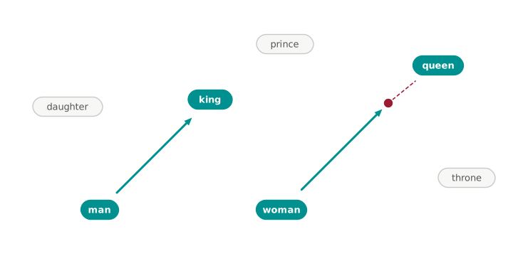
In the diagram, the two teal arrows represent the two approximately equal difference vectors. The cardinal dot at the head of the second arrow is where the arithmetic lands: near “queen” without landing on it, which is why we search for a nearest neighbor rather than expect an exact hit. The search excludes the three input words, and the arithmetic fails for many other relations. It is an observed property of these embeddings, not a guarantee of the objective.

Low-rank Weight Updates

The next lecture applies the low-rank tool to a different matrix: LoRA approximates the update that an already-trained network’s weight matrix needs to learn a new task.

Problem 16 returns to the linear autoencoder and compares the coordinate symmetries left by reconstruction, Euclidean distance, and dot-product objectives. An optional extension asks the same question for cosine similarity. The surviving transformations determine which geometric claims are identifiable and why an individual coordinate has no fixed meaning.

An embedding is optimal only relative to its training objective, so its evaluation should measure the structure that objective preserves.