Demo: Word Embeddings with PCA

We will compress word co-occurrence profiles and see what the embedding dimension changes. The counts below are illustrative, with pairs of words that share contexts. They are not measurements from a corpus.

Each row describes one word. After centering the columns, PCA gives an encoder \(E\), embeddings \(\mathbf Z\), and a decoder \(D\).

from pathlib import Path
import numpy as np
import matplotlib.pyplot as plt

plt.style.use(str(Path("../figure_style.mplstyle")))
words = np.array(["dog", "cat", "car", "truck", "apple", "pear", "violin", "piano"])
contexts = ["fur", "pet", "paws", "engine", "road", "wheels",
            "fruit", "sweet", "tree", "music", "strings", "notes"]
counts = np.array([
    [18, 15, 12, 0, 0, 0, 0, 0, 0, 0, 0, 0],
    [17, 14, 14, 0, 0, 0, 0, 0, 0, 0, 0, 0],
    [0, 0, 0, 16, 12, 18, 0, 0, 0, 0, 0, 0],
    [0, 0, 0, 17, 15, 19, 0, 0, 0, 0, 0, 0],
    [0, 0, 0, 0, 0, 0, 20, 12, 15, 0, 0, 0],
    [0, 0, 0, 0, 0, 0, 18, 14, 13, 0, 0, 0],
    [0, 0, 0, 0, 0, 0, 0, 0, 0, 20, 17, 15],
    [0, 0, 0, 0, 0, 0, 0, 0, 0, 21, 14, 18],
], dtype=float)
mean = counts.mean(axis=0)
X = counts - mean
U, singular, Vt = np.linalg.svd(X, full_matrices=False)
rank = np.linalg.matrix_rank(X)
print(f"{len(words)} words, {len(contexts)} context features, centered rank {rank}.")

8 words, 12 context features, centered rank 7.

Question 1: Which Context Patterns Are Similar?

Predict each word’s nearest neighbor from the count table. The distance between two rows measures how much their context profiles differ. Centering every row by the same feature means leaves these distances unchanged.

def nearest_neighbors(rows):
    distances = np.linalg.norm(rows[:, None, :] - rows[None, :, :], axis=2)
    np.fill_diagonal(distances, np.inf)
    return words[np.argmin(distances, axis=1)]

for word, neighbor in zip(words, nearest_neighbors(X)):
    print(f"{word:7s} -> {neighbor}")

dog     -> cat
cat     -> dog
car     -> truck
truck   -> car
apple   -> pear
pear    -> apple
violin  -> piano
piano   -> violin

Question 2: Can Two Coordinates Keep Those Relationships?

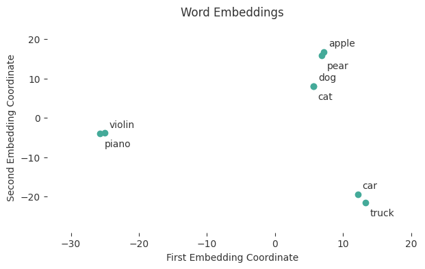
PCA chooses two directions that minimize reconstruction error. Predict whether these two coordinates will preserve the nearest neighbors, then compare the original profiles with the embeddings. The labels identify words in the plot.

k = 2
V_k = Vt[:k].T

def E(X):
    return X @ V_k

def D(Z):
    return Z @ V_k.T

Z = E(X)
print("Word     Original neighbor   Embedding neighbor")
for word, original, embedded in zip(words, nearest_neighbors(X), nearest_neighbors(Z)):
    print(f"{word:7s}  {original:17s}   {embedded}")

fig, ax = plt.subplots(figsize=(7, 4))
ax.scatter(Z[:, 0], Z[:, 1])
for i, (word, point) in enumerate(zip(words, Z)):
    offset = (5, 6) if i % 2 == 0 else (5, -14)
    ax.annotate(word, point, xytext=offset, textcoords="offset points")
ax.margins(.2)
ax.set(title="Word Embeddings", xlabel="First Embedding Coordinate", ylabel="Second Embedding Coordinate")
plt.show()

Word     Original neighbor   Embedding neighbor
dog      cat                 cat
cat      dog                 dog
car      truck               truck
truck    car                 car
apple    pear                pear
pear     apple               apple
violin   piano               piano
piano    violin              violin

Question 3: What Does the Decoder Lose?

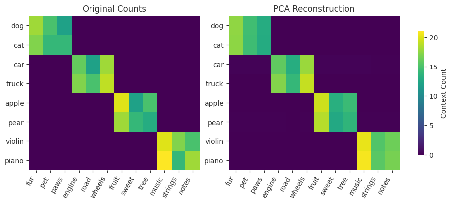
Change \(k\) below, from one through the centered matrix’s rank. Predict which context patterns will be hardest to reconstruct. Compare the measured counts with the decoder’s reconstruction, adding back the column means to return to count units.

The measured squared error should agree with the discarded squared singular values. Keeping more coordinates reduces reconstruction error, but nearest-neighbor relationships need not improve at every step.

k = 3  # Change this and rerun this cell.
assert 1 <= k <= rank
V_k = Vt[:k].T
Z = E(X)
X_hat = D(Z)
reconstructed = X_hat + mean
measured_error = np.sum((X - X_hat) ** 2)
tail_error = np.sum(singular[k:] ** 2)
assert np.isclose(measured_error, tail_error)
print(f"{k} coordinates: squared reconstruction error {measured_error:.3f}")
print(f"Discarded squared singular values: {tail_error:.3f}")
retained = np.sum(nearest_neighbors(X) == nearest_neighbors(Z))
print(f"Original nearest neighbors retained: {retained}/{len(words)}")

fig, axes = plt.subplots(1, 2, figsize=(9, 4), constrained_layout=True)
for ax, values, title in zip(axes, [counts, reconstructed], ["Original Counts", "PCA Reconstruction"]):
    image = ax.imshow(values, cmap="viridis", vmin=0, vmax=counts.max(), aspect="auto")
    ax.set_xticks(range(len(contexts)), contexts, rotation=60, ha="right")
    ax.set_yticks(range(len(words)), words)
    ax.set_title(title)
fig.colorbar(image, ax=axes, label="Context Count", shrink=.8)
plt.show()

3 coordinates: squared reconstruction error 20.222
Discarded squared singular values: 20.222
Original nearest neighbors retained: 8/8

The decoder is trained to approximate context counts. It has no separate rule saying that animal words or instrument words must be neighbors. The groups in this example come from the shared count patterns we supplied.

For a final comparison, increase one context column’s counts in the setup and rerun the notebook. Does giving that context more weight change which relationships survive compression?