Finetuning (LoRA)

Last lecture compressed data into a low-rank embedding: a dataset is a matrix, one row per point, and its best rank-\(k\) approximation is a useful summary of every row. The same tool can describe the change in a network’s weights when we adapt it to a new task.

Finetuning a huge pretrained model may require an update that uses only a few of the weight matrix’s available directions. LoRA builds that assumption into the parameterization.

The Pretrain-then-Finetune Paradigm

Modern practice rarely trains a network from scratch for every task. A model is pretrained once on a broad task with abundant data (predict the next word on a huge slice of the internet, say), and then finetuned: trained further, usually briefly, on a smaller task-specific dataset. Pretraining is where nearly all the compute goes. Finetuning makes adaptation feasible with limited compute and a few hundred labeled examples.

The class demo runs a miniature version of exactly this: pretrain a small network on upright MNIST digits, then hand it the same digits rotated \(90^\circ\). Accuracy collapses to barely above chance. Pretraining plainly learned something, but not something that survives a rotation. Finetuning is the repair, and the question is how many weights it has to touch.

What Full Finetuning Costs

The obvious repair is to unfreeze every parameter and run gradient descent on the new data. Its cost has almost nothing to do with the forward pass. We analyze one weight matrix: \[ \mathbf{W} \in \mathbb{R}^{d\times k} . \] It maps a layer input \(\mathbf{x}\in\mathbb{R}^k\) to the output \(\mathbf{W}\mathbf{x}\in\mathbb{R}^d\). Training \(\mathbf{W}\) with Adam, from the Gradient Descent lecture, means holding four arrays of that same shape at once: the weights, their gradient, Adam’s smoothed gradient, and Adam’s smoothed squared gradient. So the memory one trainable matrix demands is four times its entry count: \[ 4dk \text{ numbers} . \] Only the first of the four arrays is the model; the other three exist purely because we intend to change it, and they appear whether the finetuning dataset has ten examples or ten million. At \(d = k = 4096\), a modest hidden dimension by modern standards, those four arrays already total about \(67\) million numbers, one matrix out of the hundreds inside a transformer.

Memory accounting per matrix does not include the cost of transferring updated parameters across machines. Every task we finetune for produces its own complete copy of the network, so ten specialized models mean ten full sets of weights to store and to load.

Both costs exist only because every parameter is trainable. We now determine which part of the network must change.

The Empirical Low-Rank Structure of Weight Updates

To answer that, look at what finetuning does when we let it do anything. Write \(\Delta\mathbf{W}\) for the total change one weight matrix undergoes over a finetuning run: \[ \Delta\mathbf{W} = \mathbf{W}^{\mathrm{finetuned}} - \mathbf{W} \in \mathbb{R}^{d\times k} . \] Gradient descent was free to move all \(dk\) entries independently, and it did.

The empirical observation behind today’s lecture is that \(\Delta\mathbf{W}\) nevertheless tends to have low intrinsic rank: nearly all of its Frobenius energy sits in a handful of singular directions, far fewer than the \(\min(d,k)\) available. This is a measurement rather than a theorem, and the class demo takes it directly: on the pretrained network’s output layer, \(\mathbf{W}\in\mathbb{R}^{10\times 128}\), the update has at most \(10\) singular values to spread its energy over.

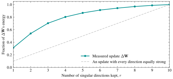
In the plot, the teal curve is the fraction of \(\Delta\mathbf{W}\)’s Frobenius energy captured by its top \(r\) singular directions, and the gray dashed line is an even spread across all ten; the measured curve sits well above it. The update is tilted: no single direction explains it, but a small budget of directions already recovers most of it. That tilt is exactly the shape the Low-rank Approximation lecture taught us to bound. By Eckart–Young–Mirsky, the best rank-\(r\) approximation of the update leaves behind exactly the tail energy of the discarded directions: \[ \big\|\Delta\mathbf{W} - (\Delta\mathbf{W})_r\big\|_F = \sqrt{\textstyle\sum_{i>r}\sigma_i^2} , \] where \(\sigma_1\geq\sigma_2\geq\cdots\) are the singular values of \(\Delta\mathbf{W}\) and \((\Delta\mathbf{W})_r\) is its truncated SVD. Our \(10\times 128\) layer has only ten directions to spread over; the published measurements that motivated LoRA, on matrices with \(d\) and \(k\) in the thousands, find the same tilt with far more room to exploit it.

If the update we want lives mostly in \(r\) directions, there is no reason to spend \(dk\) parameters searching for it. We should parameterize those \(r\) directions directly.

LoRA’s Factorization

LoRA (low-rank adaptation) does exactly that. Freeze the pretrained matrix \(\mathbf{W}\) and represent the update as a product of two thin matrices: \[ \Delta\mathbf{W} = \mathbf{B}\mathbf{A}, \qquad \mathbf{B}\in\mathbb{R}^{d\times r}, \quad \mathbf{A}\in\mathbb{R}^{r\times k}, \quad r \ll \min(d,k) . \] What this factorization can express is exactly the matrices of rank at most \(r\): the product has rank at most \(r\), and every such matrix can be written this way. The outer-product form from the Linear Algebra lecture says what the two factors are actually storing: \[ \mathbf{B}\mathbf{A} = \sum_{i=1}^r \mathbf{b}_i\mathbf{a}_i^\top , \] where \(\mathbf{b}_i\in\mathbb{R}^d\) is the \(i\)th column of \(\mathbf{B}\) and \(\mathbf{a}_i^\top\in\mathbb{R}^{1\times k}\) is the \(i\)th row of \(\mathbf{A}\): \(r\) output directions paired with \(r\) input directions, and nothing else.

The layer’s forward pass gains exactly one extra term: \[ \mathbf{h} = \mathbf{W}\mathbf{x} + \mathbf{B}\mathbf{A}\mathbf{x} \in \mathbb{R}^d , \] and only \(\mathbf{B}\) and \(\mathbf{A}\) receive gradients; \(\mathbf{W}\) never moves.

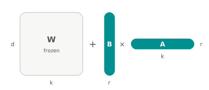
In the plot, the gray block is \(\mathbf{W}\), frozen, and the two teal strips are everything LoRA trains; the strips are drawn thin because \(r\) is small next to both \(d\) and \(k\).

The standard initialization sets one factor to zero and the other to small random values: \[ \mathbf{B} = \mathbf{0}, \qquad \mathbf{A} \text{ small and random} , \] so \(\Delta\mathbf{W} = \mathbf{B}\mathbf{A} = \mathbf{0}\) before the first step and training starts exactly at the pretrained model. We cannot set both factors to zero. The loss reaches \(\mathbf{B}\) and \(\mathbf{A}\) only through their product, so the gradient with respect to either factor carries the other factor as a multiplier. Zero out both and both gradients vanish, leaving a model that can never move.

With \(\mathbf{B}=\mathbf{0}\), the gradient with respect to \(\mathbf{A}\) vanishes at initialization even though the gradient with respect to \(\mathbf{B}\) does not. On the first step, only \(\mathbf{B}\) changes, along a direction filtered through the random initial \(\mathbf{A}\).

Counting the Savings

We count the savings at \(d = k = 4096\) and rank \(r = 8\). Full finetuning trains every entry of the matrix: \[ dk = 4096\times 4096 = 16{,}777{,}216 \text{ parameters} . \] LoRA trains only the two strips, \(d\times r\) and \(r\times k\): \[ r(d+k) = 8\times(4096+4096) = 65{,}536 \text{ parameters} , \] a factor of \(256\) fewer. The frozen count \(dk\) grows quadratically in the matrix’s dimensions while the trainable count \(r(d+k)\) grows only linearly, so at a fixed rank the saving grows the wider the matrix.

Optimizer memory falls in step, since Adam’s three auxiliary arrays are now sized to the trainable parameters alone: about \(3r(d+k) \approx 197{,}000\) numbers against \(3dk \approx 50\) million. Per-task storage falls the same way: a finetuned adapter is \(r(d+k)\) numbers per matrix instead of a fresh copy of the whole network.

Be clear about what does not get cheaper. \(\mathbf{W}\) is still stored, every forward pass still multiplies by it, and the backward pass still propagates through it to reach earlier layers. LoRA saves optimizer state and per-task storage, not the arithmetic of running the network.

Saving memory is worth little if the adapter makes the finished model slower to run.

Merging Costs Nothing at Inference

Once training finishes, \(\mathbf{B}\) and \(\mathbf{A}\) are fixed numbers, so their product is a fixed \(d\times k\) matrix, exactly the shape of \(\mathbf{W}\). Compute the sum once, offline: \[ \mathbf{W}' = \mathbf{W} + \mathbf{B}\mathbf{A} \in \mathbb{R}^{d\times k} , \] and deploy \(\mathbf{W}'\) as though it had always been the layer’s weight matrix. The served model then has exactly the architecture, exactly the parameter count, and exactly the arithmetic of the original.

Count the alternative. Keeping the factors separate and evaluating \(\mathbf{W}\mathbf{x} + \mathbf{B}(\mathbf{A}\mathbf{x})\) on every forward pass costs \(dk\) multiply-adds for the frozen part, then \(rk\) for \(\mathbf{A}\mathbf{x}\) and \(dr\) for multiplying that by \(\mathbf{B}\): \[ dk + r(d+k) \quad \text{against} \quad dk . \] At \(d = k = 4096\) and \(r = 8\) the extra term is under half a percent of the total, but it is also two additional small matrix multiplications in every adapted layer, dominated by launch overhead rather than arithmetic. Merging removes the question entirely, at the cost of one offline addition of two \(d\times k\) matrices.

(Merging is not always what we want. A server that holds one frozen \(\mathbf{W}\) plus many small adapters can answer requests for different tasks inside a single batch, which a merged \(\mathbf{W}'\), committed to one task, cannot. The real choice is between zero added latency for one task and one shared copy of the model for many.)

Both counts above assumed a value of \(r\); choosing it is the last thing left.

Rank and Scale as Hyperparameters

The rank \(r\) trades expressiveness against cost. Too small, and \(\mathbf{B}\mathbf{A}\) simply cannot reach whatever update the new task needs, since the tail energy left behind by the best rank-\(r\) approximation is a floor no training run can get under. Large enough, and LoRA recovers essentially all of full finetuning’s benefit at a fraction of its memory. Typical values in practice are surprisingly small, \(r\in\{4,8,16,32,64\}\) for matrices with \(d\) and \(k\) in the thousands.

Implementations also scale the adapter’s contribution by a constant before adding it: \[ \mathbf{h} = \mathbf{W}\mathbf{x} + \frac{s}{r}\,\mathbf{B}\mathbf{A}\mathbf{x} , \] where \(s > 0\) is a fixed hyperparameter (the original paper writes it \(\alpha\), but we reserve \(\alpha\) for the learning rate). Doubling \(r\) doubles the number of outer products in \(\mathbf{B}\mathbf{A} = \sum_i \mathbf{b}_i\mathbf{a}_i^\top\), and so roughly doubles the size of the adapter’s contribution; dividing by \(r\) cancels that, so a learning rate tuned at one rank stays sensible at another. This scaling simplifies hyperparameter search but does not affect the low-rank parameterization.

The class demo compares LoRA with full finetuning on the rotated-digit task. With limited finetuning data, the rank constraint also acts as a regularizer; increasing the dataset narrows LoRA’s advantage.

Ordinary gradient descent is not guaranteed to find the best rank-\(r\) correction. Problem 17 audits the tempting claim that this random rank-\(r\) first step is already close to the best rank-\(r\) gradient approximation. Expected captured energy supports a limited average-case statement, while a carefully aligned low-rank gradient exposes the worst-case gap.

LoRA kept gradient descent as it was and restricted the parameters it may touch; Muon keeps every parameter and asks whether gradient descent, applied to a weight matrix, should treat it as a flat list of numbers at all.