Convolutional Networks
Previous networks in this course were fully connected, with every neuron wired to every neuron in the next layer. This unit is about architectures, the wiring decisions made before a single gradient step is taken. Convolution builds the translation symmetry of images into that wiring.
The Cost of Full Connectivity
Start with the accounting. A modest \(256\times 256\) grayscale photograph, flattened the way our fully connected networks require, is a vector with \(d = 65{,}536\) entries. A single fully connected layer from that vector to a hidden layer of the same size has \(65{,}536^2 \approx 4.3\) billion weights, about \(17\) GB of parameters for one layer, before we have detected a single whisker.
A fully connected layer also ignores the spatial structure of its inputs. A fully connected layer does not encode pixel adjacency: shuffling every image’s pixels with one fixed permutation leaves the function class unchanged because nothing in \(\mathbf{W}\mathbf{x}\) depends on which entries of \(\mathbf{x}\) sit next to each other. And whatever the layer learns about whiskers in the top-left corner, it learns with weights that touch only top-left pixels; the same whiskers in the bottom-right are, to this layer, an unrelated pattern to be relearned from scratch.
Local Connectivity and Weight Sharing
Images have local structure, and the same pattern can appear at any position. Convolutional networks build both facts directly into the wiring, as two constraints on the dense layer:
- Local connectivity: each output neuron looks only at a small window of adjacent inputs, rather than the whole signal.
- Weight sharing: every window is processed by the same small set of weights.
We start with the simplest case: a one-dimensional signal \(\mathbf{x}\in\mathbb{R}^6\) and a window of size three. The shared weights \(\mathbf{w} = (w_1, w_2, w_3) \in \mathbb{R}^3\) are called a kernel (or filter), and sliding it across the signal is called a convolution: \[ y_i = \sum_{j=1}^{3} w_j \, x_{i+j-1} = w_1 x_i + w_2 x_{i+1} + w_3 x_{i+2}, \qquad i = 1, \ldots, 4. \]
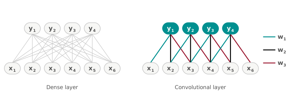
In the plot, the dense layer on the left spends \(6\times 4 = 24\) weights wiring every input to every output, while the convolutional layer on the right draws only three distinct colors: the teal, black, and cardinal edges are \(w_1\), \(w_2\), and \(w_3\), repeating at every output.
The kernel \((-1, 0, 1)\) subtracts the window’s left entry from its right, so it returns zero on a flat stretch and a large magnitude where the signal changes abruptly.
Claim: Sliding the kernel \(\mathbf{w} = (-1, 0, 1)\) across the signal \(\mathbf{x} = (1, 1, 1, 5, 5, 5)\) produces the output \(\mathbf{y} = (0, 4, 4, 0)\).
Solution to the class exercise
Slide the window one position at a time, taking the dot product of the kernel with the three entries under it: \[\begin{align} y_1 &= (-1)(1) + (0)(1) + (1)(1) = 0, \\ y_2 &= (-1)(1) + (0)(1) + (1)(5) = 4, \\ y_3 &= (-1)(1) + (0)(5) + (1)(5) = 4, \\ y_4 &= (-1)(5) + (0)(5) + (1)(5) = 0. \end{align}\]The prediction was right, and the reason shows in symbols: \[ y_i = (-1)x_i + (0)x_{i+1} + (1)x_{i+2} = x_{i+2} - x_i, \] a discrete difference: the kernel responds to the signal’s change across the window, not its level. A kernel that responds to change is an edge detector, and it detects the edge wherever it happens to be, because the same weights visit every position.
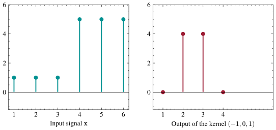
In the plot, the output is zero on the flat stretches and \(4\) where the window straddles the jump. The same computation has a matrix form. Stacking the four dot products into the matrix equation \(\mathbf{y} = \mathbf{C}\mathbf{x}\) gives a convolution matrix: \[ \mathbf{C} = \begin{bmatrix} w_1 & w_2 & w_3 & 0 & 0 & 0 \\ 0 & w_1 & w_2 & w_3 & 0 & 0 \\ 0 & 0 & w_1 & w_2 & w_3 & 0 \\ 0 & 0 & 0 & w_1 & w_2 & w_3 \end{bmatrix} \in \mathbb{R}^{4\times 6}, \] a perfectly ordinary linear layer of the kind we have used all semester, with almost no freedom left in its matrix: locality forces the zeros, and weight sharing forces each diagonal to be constant. Twenty-four entries, three free numbers. That is a large saving, but a window of size three sees almost nothing at once, so we should ask what the constraints cost.
Parameter Efficiency and the Receptive Field
The in-class exercise finishes the accounting.
Claim: Mapping \(\mathbb{R}^6\) to \(\mathbb{R}^4\) costs a dense layer \(24\) weights and a 3-tap convolution \(3\), and stacking a second 3-tap layer grows each final output’s receptive field (the set of inputs that can influence it) from \(3\) inputs to \(5\).
Solution to the class exercise
The dense layer needs one weight per input–output pair: \(6 \times 4 = 24\) (ignoring biases). The convolutional layer needs exactly its kernel, \(3\) weights, no matter how long the signal is; the same kernel would process \(6\) entries or \(6\) million. For the receptive field, stack a second 3-tap convolution on top of \(\mathbf{y}\), giving a second-layer output \(\mathbf{z}\in\mathbb{R}^2\). Its first entry \(z_1\) reads \(y_1, y_2, y_3\), and those read the inputs \(\{x_1,x_2,x_3\}\), \(\{x_2,x_3,x_4\}\), and \(\{x_3,x_4,x_5\}\) respectively, so the union is \(\{x_1,\ldots,x_5\}\): five inputs.Each additional layer extends the reach by one window’s width minus one, so the receptive field after \(L\) stacked layers of width-\(k\) kernels is: \[ L(k-1) + 1 . \] For our 3-tap kernels that is \(2L+1\), which grows only linearly in depth.
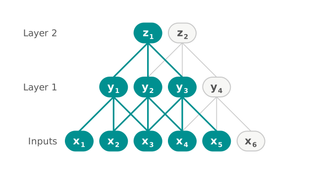
In the plot, the teal path traces every route from the inputs to one second-layer output: three layer-one neurons, five inputs. Each convolutional layer has a local receptive field. Depth expands that field while each layer retains a small parameter count. Collecting the counts in one place:
| Layer | Weights |
|---|---|
| Dense, \(\mathbb{R}^6 \to \mathbb{R}^4\) | 24 |
| 3-tap convolution, any signal length | 3 |
| Dense, \(256\times256\) image to same size | \(\approx 4.3\) billion |
| \(5\times 5\) convolution, 8 kernels (the demo’s first layer) | 208 |
The last row uses a square window and eight kernels in parallel.
Images: Channels and Feature Maps
Everything above generalizes to two dimensions by letting the window be a small square. A \(k\times k\) kernel slides over every position of the image, taking a dot product with the \(k \times k\) patch beneath it, and the grid of outputs is called a feature map: an image of where the kernel’s pattern occurs. One kernel can only detect one pattern, so a convolutional layer learns many kernels in parallel (say \(8\)), and the \(8\) feature maps stack into the layer’s channels.
The next layer’s kernels then read all of the incoming channels at once: a \(5\times 5\) kernel on an \(8\)-channel input is really a \(5\times5\times8\) block of weights. Writing \(c_{\text{in}}\) and \(c_{\text{out}}\) for the number of incoming and outgoing feature maps and \(k\) for the kernel width, the layer’s parameter count is: \[ c_{\text{out}}\left(k^2 c_{\text{in}} + 1\right), \] one \(k\times k \times c_{\text{in}}\) block plus one bias for each of the \(c_{\text{out}}\) maps. The color channels of an RGB photograph enter the same way, as an input with \(c_{\text{in}}=3\). The count does not contain the image size. A convolutional layer therefore has the same number of parameters on a thumbnail and on a billboard. The image’s size is still free to change from layer to layer, though, and three bookkeeping knobs decide how.
Stride, Padding, and Pooling
Padding addresses the shrinkage we just saw (\(6\) inputs became \(4\) outputs): surround the input with a border of zeros so the window can center on every position and the output keeps the input’s size. (A second convention wraps the signal around a circle instead, so that the window sliding off the right edge re-enters on the left. Problem 19 lives entirely in this circular world.) Stride slides the window more than one position at a time; stride \(2\) halves the output’s width and height. Pooling shrinks it without any parameters at all: max-pooling over \(2\times 2\) blocks keeps only the strongest response in each block, shrinking each feature map (so receptive fields grow twice as fast above) and making the network indifferent to which pixel within the block fired.
Translation Equivariance
Because the same kernel visits every position, shifting the input shifts the output correspondingly: convolve-then-shift equals shift-then-convolve. This property is called translation equivariance. The network does not need separate examples to learn that the same pattern can occur at different positions. (Equivariance means the output moves with the input, not yet invariance, where the output ignores the shift entirely; averaging a feature map over all positions, as our demo network does before its final layer, is the standard step from one to the other.)
The one place the equality can fail is the boundary, where a shifted signal loses an entry off the end of our \(4\times 6\) matrix \(\mathbf{C}\); wrap the signal around a circle, making \(\mathbf{C}\) square, and the property becomes an algebraic identity. Write \(\mathbf{S} \in \mathbb{R}^{6\times 6}\) for the shift matrix, which rotates a signal one position, so that \((\mathbf{S}\mathbf{x})_i = x_{i+1}\) with indices read around the circle. Then circular convolution commutes with the shift: \[ \mathbf{C}\mathbf{S} = \mathbf{S}\mathbf{C} . \] Apply both sides to a signal: \(\mathbf{C}(\mathbf{S}\mathbf{x}) = \mathbf{S}(\mathbf{C}\mathbf{x})\) says that convolving a shifted signal and shifting a convolved signal are the same computation, and it says it for every kernel at once. Problem 19 proves that a linear map commutes with cyclic shifts exactly when it is a circular convolution. Fourier diagonalization is supplied as a consequence, then used to recover the convolution eigenvalues and connect weight sharing to FFT computation. The same shift-respecting structure appears in rotary positional embeddings, where attention scores form a Toeplitz pattern.
What the Kernels Learn
The class demo compares a small convolutional network with a fully connected network on MNIST. The convolutional model reaches similar accuracy with far fewer parameters.
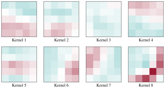
The plot shows the first layer’s eight learned kernels, teal for positive weights and cardinal for negative. Almost every one is an oriented light-to-dark transition: an edge detector, the two-dimensional version of the \((-1, 0, 1)\) kernel we applied by hand. The objective did not specify edge detection; the learned kernels nevertheless respond to oriented transitions.
Because the network ends with a global average and a linear layer, we can also see where it looks. Write \(\mathbf{A}_k \in \mathbb{R}^{7\times 7}\) for the \(k\)-th feature map of the last convolutional layer, \([\mathbf{A}_k]_p\) for its value at one of the \(49\) spatial positions \(p\), \(w_{c,k}\) for the weight that map receives in the final layer, and \(s_c\) for the score the network assigns to class \(c\). The network averages each map and then combines them, and we exchange the two sums: \[\begin{align} s_c &= \sum_{k=1}^{16} w_{c,k} \left(\frac{1}{49}\sum_{p} [\mathbf{A}_k]_p\right) \\ &= \frac{1}{49}\sum_{p} \sum_{k=1}^{16} w_{c,k}\,[\mathbf{A}_k]_p \\ &= \frac{1}{49}\sum_{p} \left[\mathrm{CAM}_c\right]_p , \end{align}\] where the first line is the definition of the network’s head, the second pulls the constant \(1/49\) out and swaps two finite sums, and the third names the image whose \(49\) entries we just added up: \[ \mathrm{CAM}_c = \sum_{k=1}^{16} w_{c,k} \, \mathbf{A}_k \in \mathbb{R}^{7\times 7}. \]
The class score is the spatial average of this image, so \([\mathrm{CAM}_c]_p\) is the contribution from position \(p\) to the score for class \(c\). This class activation map costs no gradients and no extra training.
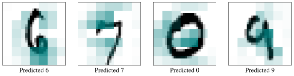
In the plot, the teal heat sits on each digit’s most distinctive strokes: the lower loop of the \(6\), the top bar of the \(7\). The demo also computes a class activation map for a class that is not present in the image.
Convolution assumes that the interactions that matter are local. For images it holds, but consider the sentence “The cat, which had been hiding under the porch all morning, was hungry.” The words “cat” and “hungry” need to interact, and they are eleven positions apart. Next lecture removes the constraint: self-attention lets every position interact with every other in a single layer, with strengths computed from the data rather than fixed by the wiring. Such a layer has no positional information; a later lecture adds it explicitly.