Convolutional Networks
An edge can appear anywhere in an image. If we train a fully connected network to recognize it on the left, the network has separate weights for recognizing the same edge on the right. We’d like to reuse what it learned. The same issue appears in audio and other signals: a useful local pattern can occur at many positions.
A convolutional layer applies one learned rule throughout the input. The rule looks at a small neighborhood, so we can apply it to images much larger than the examples used to learn it. This is another way to use matrix structure. Here, we constrain the layer itself by making many of its weights equal.
We’ll build a shared local filter, see how several layers combine distant information, and derive what happens when the input shifts.
Receptive Fields
Locality saves parameters, but one layer cannot immediately combine distant evidence. Depth supplies that reach. The receptive field of an output is the set of original inputs that can influence it.
A later layer combines neighboring outputs whose input windows overlap. Their union reaches farther than any single window.
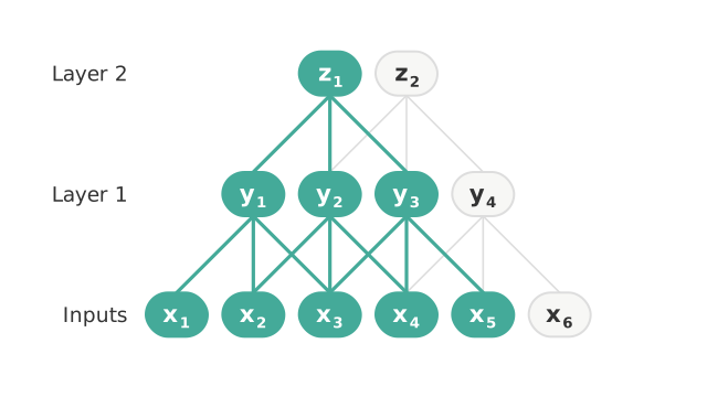
The receptive-field width depends on both kernel width and depth.
Claim: On an unbounded signal with stride one, no dilation, integer \(k\geq1\), and integer \(L\geq0\), the maximum receptive-field width after \(L\) width-\(k\) layers is \[ 1+L(k-1). \]
Proof
Before any convolution, one representation depends on one input, so \(R^{(0)}=1\). If an output after \(l\) layers can depend on a contiguous block of width \(R^{(l)}\), the next width-\(k\) layer reads \(k\) adjacent such outputs. Consecutive blocks start one input position apart, so their union begins with the first block and extends \(k-1\) positions beyond it. Therefore \[ R^{(l+1)}=R^{(l)}+(k-1). \] Starting from \(R^{(0)}=1\) and applying the recurrence \(L\) times gives \(R^{(L)}=1+L(k-1)\). This proves the formula.
A single output in this stack cannot combine evidence separated by more than \(L(k-1)\) positions. A later operation that pools across the whole signal can combine more, but the local stack alone has limited reach.
Pointwise activations change the values but do not enlarge this field: each activation reads only the value at its own position. An input inside the field may have little effect because of learned weights or activations. An input outside it cannot affect this output at all.
This distinction matters when choosing depth. A local pattern may be visible to one layer, while combining several parts of an object requires a larger region. Increasing the kernel width or adding layers expands that region. Strides, which skip positions, and dilation, which spaces out kernel entries, change the formula above. We have kept both out of this calculation to isolate the effect of depth.
Translation Equivariance
We wanted the same detector to work wherever a pattern appears. Weight sharing gives a precise version of that idea. Away from boundaries, shifting the input shifts every local window and therefore shifts the output by the same amount. This is translation equivariance: \[ \operatorname{Conv}(\operatorname{Shift}(\mathbf x)) =\operatorname{Shift}(\operatorname{Conv}(\mathbf x)). \] Equivariance means the representation moves predictably with the input. It differs from invariance, in which the final answer does not move at all. A classifier can obtain approximate shift invariance later by pooling or averaging spatial responses, but the convolutional layers first preserve where a feature was found.
Segmentation usually needs equivariance because shifting an object should shift its predicted mask. Classification often seeks invariance because the final label should remain unchanged.
Boundaries require a convention because an ordinary shift can discard data. Circular indexing temporarily removes that ambiguity, so the following result isolates what weight sharing itself guarantees before a padding rule complicates the edges.
Claim: With circular wraparound, a shared convolution \(\mathbf C\) commutes with every integer shift \(\mathbf S_q\): \[ \mathbf C\mathbf S_q=\mathbf S_q\mathbf C. \]
Proof
Index a length-\(n\) signal modulo \(n\), so \(x_{i+n}=x_i\) for every integer \(i\). For any integer \(q\), define the circular shift by \((\mathbf S_q\mathbf x)_i=x_{i-q}\) for \(i=1,\ldots,n\). The circular convolution has \(n\) outputs and is a weighted sum of shifts: \[ \mathbf C=\sum_{j=1}^k w_j\mathbf S_{1-j}, \qquad \mathbf C,\mathbf S_q\in\mathbb R^{n\times n}, \] because \((\mathbf S_{1-j}\mathbf x)_i=x_{i+j-1}\). Shifts commute: for any integers \(p,q\), composing them adds their offsets, so \(\mathbf S_p\mathbf S_q=\mathbf S_{p+q}=\mathbf S_q\mathbf S_p\). Distributing through the finite sum therefore gives \[ \mathbf C\mathbf S_q=\sum_{j=1}^k w_j\mathbf S_{1-j}\mathbf S_q=\sum_{j=1}^k w_j\mathbf S_q\mathbf S_{1-j}=\mathbf S_q\mathbf C. \] Weight sharing makes the coefficients \(w_j\) independent of position, which is what lets convolution use this fixed combination of shifts.
The same pointwise activation at every position also commutes with a shift. We can therefore stack these layers without losing the property, as long as the boundary and stride conventions preserve it.
The comparison below uses a circular input shift in both cases.
A circular convolution commutes with a circular shift. Zero padding changes boundary neighborhoods and can break that equality.
Circular convolution respects the circular shift. Zero padding creates an edge where the operations can disagree.
Zero padding or cropping breaks exact shift symmetry at an ordinary image boundary, while the shared kernel remains equivariant in the interior.
Sharing a kernel lets us learn a pattern once and apply it across positions. The cost of keeping each layer local is that distant inputs need several layers to interact. In the next reading, attention will let an output choose directly among inputs throughout a sequence.