Self-attention
Last lecture ended on a sentence: “The cat, which had been hiding under the porch all morning, was hungry.” The words “cat” and “hungry” need to interact, and they sit eleven positions apart. Our receptive-field formula \(2L+1\) says a 3-tap convolution needs six stacked layers before those two words so much as touch, and language plants dependencies at every distance. Convolution assumed the interactions that matter are local, and today we drop that assumption: self-attention connects every position to every other in a single layer, with connection strengths computed on the fly from the data rather than fixed in a weight matrix.
Self-attention lets each token compute which other tokens contribute to its output. The comparisons must stay at a scale where the softmax responds, and content comparisons alone contain no positional information.
From Text to Vectors
Neural networks eat vectors, so the first step is turning text into them. A tokenizer splits text into tokens, pieces drawn from a fixed vocabulary of \(m\) types. (For us a token is a word; real systems use subword pieces, so that even a misspelled or invented word decomposes into known chunks.) Each token type then gets a learned token embedding, and the whole vocabulary’s worth of them is collected into one matrix: \[ \mathbf{E}\in\mathbb{R}^{m\times d}, \qquad \text{row } t \text{ of } \mathbf{E} \text{ is the } d\text{-dimensional vector for token type } t. \] Tokenizing “the cat was hungry” and looking up each token’s row produces vectors \(\mathbf{x}_1, \ldots, \mathbf{x}_n \in \mathbb{R}^d\), which we stack as the rows of \(\mathbf{X}\in\mathbb{R}^{n\times d}\). Here \(n\) is the sequence length and \(d\) the embedding dimension, so \(\mathbf{X}\) plays the role the design matrix played all semester, with one row per token instead of per data point. These embeddings are parameters like any others, trained by gradient descent; the Embeddings lecture showed us the geometry they learn, where similar words sit close together and directions carry meaning.
The input is \(n\) vectors in \(\mathbb{R}^d\), each initially computed independently of the others. The question is what a layer on such a sequence should do.
Queries, Keys, and Values
For the word “hungry” to use information about its subject, it needs to score the other tokens and retrieve content from the highest-scoring ones.
Self-attention implements this with three learned linear projections of each token’s embedding. Fix weight matrices \(\mathbf{W}_Q, \mathbf{W}_K \in \mathbb{R}^{d\times d_k}\) and \(\mathbf{W}_V\in\mathbb{R}^{d\times d_v}\), where \(d_k\) is the dimension for comparing queries with keys and \(d_v\) the dimension of the content passed along. Token \(i\) then computes three vectors:
- a query \(\mathbf{q}_i = \mathbf{W}_Q^\top \mathbf{x}_i \in \mathbb{R}^{d_k}\), which determines what token \(i\) matches;
- a key \(\mathbf{k}_i = \mathbf{W}_K^\top \mathbf{x}_i \in \mathbb{R}^{d_k}\), which is matched against queries; and
- a value \(\mathbf{v}_i = \mathbf{W}_V^\top \mathbf{x}_i \in \mathbb{R}^{d_v}\), which supplies token \(i\)’s content to the output.
The three matrices are the layer’s only parameters, shared across positions: every token uses the same \(\mathbf{W}_Q\), just as every window of last lecture’s convolution used the same kernel. Stacking the projections over all \(n\) tokens gives \(\mathbf{Q} = \mathbf{X}\mathbf{W}_Q \in \mathbb{R}^{n\times d_k}\), \(\mathbf{K} = \mathbf{X}\mathbf{W}_K \in \mathbb{R}^{n\times d_k}\), and \(\mathbf{V} = \mathbf{X}\mathbf{W}_V \in \mathbb{R}^{n\times d_v}\).
Scores, Softmax, and the Weighted Sum
The inner product from the Linear Algebra lecture measures how well token \(j\)’s key matches token \(i\)’s query. The attention score of query \(i\) against key \(j\) is their inner product, divided by a constant we will justify in the next section: \[ s_{ij} = \frac{\langle \mathbf{q}_i, \mathbf{k}_j\rangle}{\sqrt{d_k}}. \] The score is large when \(\mathbf{q}_i\) and \(\mathbf{k}_j\) are large and aligned, negative when they point in opposite directions, and nothing else affects it. The score does not use the positions \(i\) or \(j\) themselves, so it contains no positional information.
Scores are arbitrary real numbers, but “how much should token \(i\) listen to each token” ought to be a distribution, nonnegative and summing to one. Applying the softmax from the Logistic Regression lecture across \(j\) gives the attention weights: \[ a_{ij} = \frac{e^{s_{ij}}}{\sum_{l=1}^n e^{s_{il}}}. \] The layer’s output for token \(i\) is then the value-weighted sum, one output vector per token: \[ \mathbf{o}_i = \sum_{j=1}^n a_{ij}\,\mathbf{v}_j \in \mathbb{R}^{d_v}. \] Stacking all \(n\) of those rows, with the softmax applied to each row of the score matrix, the entire layer is one formula: \[ \operatorname{Attention}(\mathbf{X}) = \operatorname{softmax}\!\left(\frac{\mathbf{Q}\mathbf{K}^\top}{\sqrt{d_k}}\right)\mathbf{V} \in \mathbb{R}^{n\times d_v}. \] Every output is a weighted average of the same \(n\) value vectors, and all a token gets to choose is the mixing weights. One layer can connect token \(1\) directly to token \(10{,}000\), without stacking layers to expand a receptive field.
We compute the layer by hand on the four-token core of last lecture’s sentence, “the cat was hungry”, with \(d_k = 4\) (so \(\sqrt{d_k}=2\)). Suppose the learned projections produce this query for “hungry” and these four keys: \[ \mathbf{q}_{\text{hungry}} = \begin{bmatrix} 2 \\ 0 \\ 0 \\ 0\end{bmatrix}, \qquad \mathbf{k}_{\text{the}} = \begin{bmatrix} -1 \\ 0 \\ 0 \\ 0\end{bmatrix}, \quad \mathbf{k}_{\text{cat}} = \begin{bmatrix} 2 \\ 0 \\ 0 \\ 0\end{bmatrix}, \quad \mathbf{k}_{\text{was}} = \begin{bmatrix} 0 \\ 1 \\ 0 \\ 0\end{bmatrix}, \quad \mathbf{k}_{\text{hungry}} = \begin{bmatrix} 0 \\ 0 \\ 1 \\ 0\end{bmatrix}, \] where the first coordinate represents subject agreement: the query for “hungry” aligns with the key for “cat” and points opposite the key for “the”. Take the four scores one move at a time, first the inner products and then the division by \(\sqrt{d_k} = 2\): \[\begin{align} \langle\mathbf{q}_{\text{hungry}}, \mathbf{k}_{\text{the}}\rangle &= (2)(-1) = -2, &\quad s_{\text{the}} &= -2/2 = -1, \\ \langle\mathbf{q}_{\text{hungry}}, \mathbf{k}_{\text{cat}}\rangle &= (2)(2) = 4, &\quad s_{\text{cat}} &= 4/2 = 2, \\ \langle\mathbf{q}_{\text{hungry}}, \mathbf{k}_{\text{was}}\rangle &= (2)(0) = 0, &\quad s_{\text{was}} &= 0/2 = 0, \\ \langle\mathbf{q}_{\text{hungry}}, \mathbf{k}_{\text{hungry}}\rangle &= (2)(0) = 0, &\quad s_{\text{hungry}} &= 0/2 = 0, \end{align}\] where each inner product collapses to a single product, since only the query’s first coordinate is nonzero. Exponentiating the four scores and dividing each result by their sum gives the weights: \[ (a_{\text{the}}, a_{\text{cat}}, a_{\text{was}}, a_{\text{hungry}}) \approx (0.038,\; 0.757,\; 0.102,\; 0.102). \]
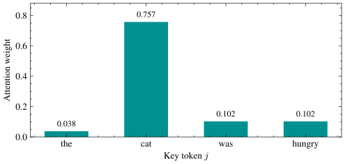
In the plot, “hungry” puts three quarters of its attention on “cat”: the layer resolved who is hungry in one step, and it would have done so at distance eleven exactly as well as at distance three. Suppose the values are \(\mathbf{v}_{\text{the}} = (0,0)\), \(\mathbf{v}_{\text{cat}} = (1,0)\), \(\mathbf{v}_{\text{was}} = (0,1)\), and \(\mathbf{v}_{\text{hungry}} = (0,1)\), with the first coordinate carrying “animal” content and the second “verb-ish” content. The output is then the weighted blend: \[ \mathbf{o}_{\text{hungry}} = 0.038 \begin{bmatrix}0\\0\end{bmatrix} + 0.757\begin{bmatrix}1\\0\end{bmatrix} + 0.102\begin{bmatrix}0\\1\end{bmatrix} + 0.102\begin{bmatrix}0\\1\end{bmatrix} \approx \begin{bmatrix}0.76\\0.20\end{bmatrix}, \] mostly the cat’s value with a whiff of verb. Nothing here is hard-coded: gradient descent chooses \(\mathbf{W}_Q\), \(\mathbf{W}_K\), and \(\mathbf{W}_V\), and which tokens attend to which is decided at runtime by the data. Problem 20 gives a concrete attention head and asks you to audit its lookup confidence before finding a task that content-only scores cannot solve.
Our worked example used \(d_k = 4\), and the scores came out around \(1\) or \(2\), right where the softmax spreads its weight. A real head has \(d_k = 64\) or more, so we should ask what happens when the head gets wide.
Scaling Scores by \(\sqrt{d_k}\)
We derive the denominator in class. At initialization, weights are scaled so that activations have roughly independent, mean-zero, unit-variance entries, which was the point of the initialization discussion in the Depth-enablers lecture. So model \(\mathbf{q}\) and \(\mathbf{k}\) as vectors of independent, mean-zero, unit-variance entries and ask how big their inner product typically is. The mechanical answer first: an inner product in \(\mathbb{R}^{d_k}\) sums \(d_k\) independent fluctuations of typical size \(1\), and independent fluctuations accumulate like \(\sqrt{d_k}\) rather than \(d_k\) because they cancel about as often as they reinforce. The claim makes that precise.
Claim: If the entries of \(\mathbf{q}, \mathbf{k} \in \mathbb{R}^{d_k}\) are independent with mean zero and variance one, then \(\mathbb{E}[\langle\mathbf{q},\mathbf{k}\rangle] = 0\) and \(\mathrm{Var}(\langle\mathbf{q},\mathbf{k}\rangle) = d_k\).
Proof of Claim
Write the inner product as a sum of products, \(\langle\mathbf{q},\mathbf{k}\rangle = \sum_{j=1}^{d_k} q_j k_j\), the same sum-of-products we analyzed for one neuron’s pre-activation in the Depth-enablers lecture, with \(q_j\) playing the weights and \(k_j\) the inputs. Each term has mean \(\mathbb{E}[q_jk_j] = \mathbb{E}[q_j]\,\mathbb{E}[k_j] = 0\), using independence to split the expectation, so the sum has mean zero by linearity of expectation. For the variance, the \(d_k\) terms are independent of each other because each uses a different pair of coordinates, so the variance-of-a-sum claim from the Probability lecture applies with every covariance term equal to zero: \[ \mathrm{Var}\left(\sum_{j=1}^{d_k} q_jk_j\right) = \sum_{j=1}^{d_k} \mathrm{Var}(q_jk_j). \] Each of those terms equals one, by the definition of variance and one more split by independence: \[ \mathrm{Var}(q_jk_j) = \mathbb{E}[(q_jk_j)^2] - \mathbb{E}[q_jk_j]^2 = \mathbb{E}[q_j^2]\,\mathbb{E}[k_j^2] - 0^2 = 1 \cdot 1 = 1 , \] where the first equality is the definition of variance, the second splits \(\mathbb{E}[q_j^2k_j^2]\) by independence and reuses the mean-zero computation above, and the third uses that a mean-zero variable’s second moment is its variance: \[ \mathbb{E}[q_j^2] = \mathrm{Var}(q_j) + \mathbb{E}[q_j]^2 = 1 + 0 = 1, \] and the same for \(k_j\). Summing \(d_k\) ones gives \(\mathrm{Var}(\langle\mathbf{q},\mathbf{k}\rangle) = d_k\).So an unscaled score has standard deviation \(\sqrt{d_k}\), growing with the head size and with nothing else: at a typical head size of \(d_k = 64\), scores of size \(\pm 8\) are routine. Dividing by \(\sqrt{d_k}\) pulls a factor of \(1/d_k\) out of the variance: \[ \mathrm{Var}\!\left(\frac{\langle\mathbf{q},\mathbf{k}\rangle}{\sqrt{d_k}}\right) = \frac{1}{d_k}\,\mathrm{Var}(\langle\mathbf{q},\mathbf{k}\rangle) = \frac{d_k}{d_k} = 1 . \] The scaled score has standard deviation \(1\) no matter the head size, which is the one property we wanted.
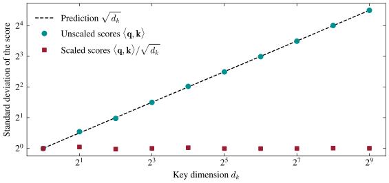
In the plot, the empirical standard deviation over \(5{,}000\) random unit-variance pairs sits on the \(\sqrt{d_k}\) prediction at every head size, while the scaled score stays flat at \(1\). The softmax responds differently when its inputs have magnitude \(1\) rather than \(8\).
Softmax Saturation and Gradients
Feed the softmax scores with gaps of \(8\) or \(16\) and it stops being a soft max: since \(e^{8} \approx 3{,}000\), the largest score takes essentially all the weight and the distribution saturates to one-hot. You might reasonably object that hard attention seems fine, even desirable. It breaks training, and the reason is the gradient. Recall how we differentiated the softmax inside the cross-entropy gradient in the Logistic Regression lecture; the same moves give the full Jacobian, which we also derive in class.
Claim: For \(\mathbf{a} = \operatorname{softmax}(\mathbf{s})\) with \(\mathbf{s}\in\mathbb{R}^n\), the Jacobian entries are \(\partial a_j/\partial s_l = a_j(\mathbb{1}[j = l] - a_l)\), and every entry tends to \(0\) as \(\mathbf{a}\) approaches a one-hot vector.
Proof of Claim
Write \(a_j = e^{s_j}/Z\) with \(Z = \sum_{l'} e^{s_{l'}}\). For \(l = j\), both the numerator and the denominator depend on \(s_j\), so the quotient rule gives: \[ \frac{\partial a_j}{\partial s_j} = \frac{e^{s_j} Z - e^{s_j} e^{s_j}}{Z^2} = a_j - a_j^2 = a_j(1 - a_j), \] where we used \(\partial Z/\partial s_j = e^{s_j}\) and then split the fraction into \(e^{s_j}/Z = a_j\) and \((e^{s_j}/Z)^2 = a_j^2\). For \(l \neq j\), the numerator \(e^{s_j}\) does not depend on \(s_l\), so only the denominator moves: \[ \frac{\partial a_j}{\partial s_l} = -\frac{e^{s_j} e^{s_l}}{Z^2} = -a_ja_l. \] The two cases combine into \(a_j(\mathbb{1}[j=l] - a_l)\), since the indicator supplies the extra \(a_j\) exactly when \(j = l\). Now let \(\mathbf{a}\) approach one-hot, say \(a_{j^*} \to 1\) and \(a_j \to 0\) for \(j \neq j^*\). Every entry of the Jacobian is a product of softmax weights: for \(j \neq j^*\) the factor \(a_j \to 0\) kills it, and for \(j = j^* = l\) the factor \((1 - a_{j^*}) \to 0\) does, so the entire Jacobian tends to the zero matrix.Every entry is a product of attention weights, so the layer’s sensitivity to its own scores is largest when the weights are spread out and smallest when one weight has already won. Whatever loss \(\mathcal{L}\) sits downstream, a score influences it only through the weights, so the chain rule routes the gradient through this Jacobian: \[ \frac{\partial \mathcal{L}}{\partial s_l} = \sum_{j=1}^n \frac{\partial \mathcal{L}}{\partial a_j}\,\frac{\partial a_j}{\partial s_l} = \sum_{j=1}^n \frac{\partial \mathcal{L}}{\partial a_j}\, a_j\big(\mathbb{1}[j=l] - a_l\big). \] Every term carries a factor of \(a_j\), so the sum approaches zero for a saturated softmax no matter how large the downstream gradient is. The gradients with respect to \(\mathbf{W}_Q\) and \(\mathbf{W}_K\) also approach zero. There, the gradient \(\mathbf{p}-\mathbf{y}\) vanished when the model was confident and correct, which is exactly when we want training to stop. Here the Jacobian vanishes whenever the softmax is confident, right or wrong, so gradient descent cannot readily change a saturated attention pattern. Without the \(\sqrt{d_k}\), a wide head can be saturated at initialization because its random scores have standard deviation \(\sqrt{d_k}\).
The class demo measures both regimes at \(d_k = 256\).
Attention Lacks Positional Information
Nothing in queries, keys, values, or inner products refers to a token’s position. Each \(\mathbf{q}_i\) is computed from \(\mathbf{x}_i\) alone, and the score \(s_{ij}\) compares content with content, as we noted when we first wrote it down. Let \(\mathbf{P}\in\mathbb{R}^{n\times n}\) be a permutation matrix that reorders the rows of \(\mathbf{X}\) (Problem 19’s shift matrix is one example), and feed the layer \(\mathbf{P}\mathbf{X}\) in place of \(\mathbf{X}\). The projections act on the right, so \(\mathbf{Q}\), \(\mathbf{K}\), and \(\mathbf{V}\) become \(\mathbf{P}\mathbf{Q}\), \(\mathbf{P}\mathbf{K}\), and \(\mathbf{P}\mathbf{V}\), and we can take the layer apart one step at a time: \[\begin{align} \operatorname{Attention}(\mathbf{P}\mathbf{X}) &= \operatorname{softmax}\!\left(\frac{(\mathbf{P}\mathbf{Q})(\mathbf{P}\mathbf{K})^\top}{\sqrt{d_k}}\right)\mathbf{P}\mathbf{V} \\ &= \operatorname{softmax}\!\left(\mathbf{P}\,\frac{\mathbf{Q}\mathbf{K}^\top}{\sqrt{d_k}}\,\mathbf{P}^\top\right)\mathbf{P}\mathbf{V} \\ &= \mathbf{P}\operatorname{softmax}\!\left(\frac{\mathbf{Q}\mathbf{K}^\top}{\sqrt{d_k}}\right)\mathbf{P}^\top\mathbf{P}\mathbf{V} \\ &= \mathbf{P}\operatorname{Attention}(\mathbf{X}), \end{align}\] where the second line uses \((\mathbf{P}\mathbf{K})^\top = \mathbf{K}^\top\mathbf{P}^\top\), the third uses that conjugating by \(\mathbf{P}\) only relabels rows and columns while the row-wise softmax acts on each row’s entries regardless of their order, and the fourth uses \(\mathbf{P}^\top\mathbf{P} = \mathbf{I}\) because permutation matrices are orthogonal. Self-attention is permutation-equivariant: scramble the sentence, and the outputs are the same vectors, scrambled the same way.
Convolution’s equivariance to shifts was the inductive bias images needed. Attention is equivariant to every permutation, so “dog bites man” and “man bites dog” produce identical sets of output vectors. Convolution respects position but has a short reach; attention has unlimited reach but no sense of position. Injecting position into the embeddings resolves this problem. Rotary embeddings later produce Toeplitz attention-score matrices, a relative-position structure related to the circulant matrices in Problem 19.
A real transformer runs many such layers, several heads apiece, interleaved with the MLPs, residual connections, and normalization from the Depth-enablers lecture. Next time we assemble that full block, count what connecting everything to everything costs (\(O(n^2d)\) time and \(O(n^2)\) memory per layer), and generate text with it. Before then, Problem 20 pairs that construction with an obstruction: content alone cannot prefer the later of two identical keys. Positional information is not merely helpful for that task; it is necessary. The input scale of a softmax is a design decision: large inputs produce a concentrated distribution with gradients near zero.