Transformer
Last lecture we built a single self-attention layer: each token projects to a query, a key, and a value; the scaled dot products \(s_{ij} = \langle\mathbf{q}_i, \mathbf{k}_j\rangle/\sqrt{d_k}\) become scores; and a row-wise softmax turns them into weights \(a_{ij}\) that average the values. One softmax per token supplies only one attention pattern, although a sentence contains several relationships worth tracking at once. Attention is also permutation-equivariant and has no information about token position. The transformer addresses the first limitation with multiple attention heads and adds the components needed to train a deep generative model; positional information comes next lecture.
Multi-head Attention
When “hungry” attends to its sentence, it may need its subject (“cat”), its verb (“was”), or a nearby negation. A single softmax must express all of those needs as one distribution over the tokens, and a split between “cat” and “was” serves both badly.
The fix is to run \(h\) copies of last lecture’s layer in parallel, called heads, each learning its own notion of relevance through projections narrower than the full width: \[ \mathbf{W}_Q^{(i)}, \; \mathbf{W}_K^{(i)}, \; \mathbf{W}_V^{(i)} \in \mathbb{R}^{d \times d/h}, \qquad i = 1, \ldots, h . \] Head \(i\) runs exactly last lecture’s computation in dimension \(d_k = d_v = d/h\), on \(\mathbf{Q}^{(i)} = \mathbf{X}\mathbf{W}_Q^{(i)}\), \(\mathbf{K}^{(i)} = \mathbf{X}\mathbf{W}_K^{(i)}\), and \(\mathbf{V}^{(i)} = \mathbf{X}\mathbf{W}_V^{(i)}\), and outputs an \(n\times d/h\) matrix. Concatenating the \(h\) outputs restores an \(n\times d\) matrix, and one final square matrix \(\mathbf{W}_O\in\mathbb{R}^{d\times d}\) mixes the heads back together: \[ \operatorname{MultiHead}(\mathbf{X}) = \left[\operatorname{head}_1 \,|\, \cdots \,|\, \operatorname{head}_h\right]\mathbf{W}_O, \qquad \operatorname{head}_i = \operatorname{softmax}\!\left(\frac{\mathbf{Q}^{(i)}(\mathbf{K}^{(i)})^\top}{\sqrt{d_k}}\right)\mathbf{V}^{(i)} . \] Without \(\mathbf{W}_O\), each head would occupy its own fixed slice of the output and could not mix with the others.
Now count what the heads cost. Each of the \(h\) heads owns \(3\) matrices of shape \(d\times d/h\), so the projections together hold: \[ h \cdot 3 \cdot d \cdot \frac{d}{h} \;=\; 3 \cdot d \cdot d \;=\; 3d^2 \] parameters, and \(\mathbf{W}_O\)’s \(d^2\) entries bring the attention sublayer to \(4d^2\), with no \(h\) anywhere: heads divide the width rather than multiplying the parameters. What \(h\) does change is the number of separate softmaxes, and therefore the number of relationships one layer can track at once, each in a narrower subspace. In trained models, researchers have identified heads that track subject-verb pairs, copy the previous token, or match quotation marks. Problem 20’s induction head is a two-head circuit observed in trained language models.
Multi-head attention gives a layer many routing patterns at once, but it still only routes; nothing yet processes the information that arrives.
The Transformer Block
Hold the attention weights fixed for a moment and look at what the layer does to the values: \[ \mathbf{o}_i = \sum_{j=1}^n a_{ij}\mathbf{v}_j . \] Given the weights, this is an average, a linear function of \(\mathbf{v}_1, \ldots, \mathbf{v}_n\): the softmax is nonlinear in the scores, but no nonlinearity ever touches the content being moved, so a stack of pure attention layers would compute little more than a data-dependent sequence of linear maps.
So the transformer pairs attention with the oldest tool we have, an MLP applied to each position separately: \[ \operatorname{MLP}(\mathbf{u}) = \mathbf{W}_2^\top\,\sigma\!\left(\mathbf{W}_1^\top \mathbf{u}\right), \qquad \mathbf{W}_1 \in \mathbb{R}^{d\times d_{\text{ff}}}, \quad \mathbf{W}_2 \in \mathbb{R}^{d_{\text{ff}}\times d}, \] where \(\mathbf{u}\in\mathbb{R}^d\) is one token’s vector, \(\sigma\) is a nonlinearity such as the ReLU, and \(d_{\text{ff}}\) is a hidden width conventionally set to \(4d\). The same \(\mathbf{W}_1\) and \(\mathbf{W}_2\) are applied at every position, so the division of labor is clean: attention routes information across positions, the MLP processes it within each one.
We are about to stack dozens of these, and the Depth-enablers lecture told us what a deep stack demands: residual connections, so the gradient always has an undamaged identity path back to every layer (Problem 13’s \(2^L\)-path highway), and normalization, so every layer’s input stays well-scaled. The transformer wraps both sublayers in both tools: \[ \mathbf{X} \;\leftarrow\; \mathbf{X} + \operatorname{MultiHead}(\operatorname{LN}(\mathbf{X})), \qquad\text{then}\qquad \mathbf{X} \;\leftarrow\; \mathbf{X} + \operatorname{MLP}(\operatorname{LN}(\mathbf{X})), \] where \(\operatorname{LN}\) is layer normalization, applied to each token’s \(d\) features separately. When we met layer normalization we said it would be the standard for sequence models, and this is why: it depends on neither the sequence length nor the batch size. (We placed the normalization before each sublayer, the modern “pre-norm” arrangement; the original transformer paper, Attention Is All You Need, put it after.)
The running \(\mathbf{X}\) is a residual stream that every sublayer reads from and adds to rather than overwriting. Information added by block \(3\) is therefore still available to block \(40\). The pair of updates above is one transformer block, and a transformer is an embedding layer, \(L\) blocks stacked, and a final linear map back to the \(m\) vocabulary entries. GPT-3 stacks \(L = 96\) of them; our class demo stacks \(2\).
Stacking blocks gives a function from a sequence of tokens to a sequence of vectors. We train it for next-token prediction.
Causal Masking
The task that powers modern language models is language modeling: given tokens \(1, \ldots, i\), predict token \(i+1\). That is classification over the \(m\) vocabulary entries, so the loss is the softmax cross-entropy we derived in the Logistic Regression lecture, now with \(m\) classes and a transformer computing the scores.
Unmasked attention would let position \(i\) directly use token \(i+1\) while predicting it. A model that learns to do so has learned nothing, and it will have nothing to say at generation time, when position \(i+1\) does not exist yet. The fix is the causal mask, applied to the scores before the softmax: \[ s_{ij} \;\leftarrow\; -\infty \quad \text{for } j > i . \] Since \(e^{-\infty} = 0\), the future terms drop out of both the numerator and the denominator of the softmax, so the attention weights of query \(i\) become: \[ a_{ij} = \begin{cases} \dfrac{e^{s_{ij}}}{\sum_{l=1}^{i} e^{s_{il}}}, & j \leq i, \\[1.2em] 0, & j > i . \end{cases} \] (Do you see why the mask has to be applied to the scores rather than to the weights afterward?)
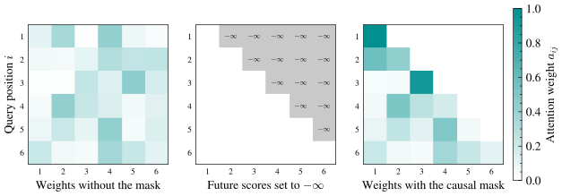
In the plot, rows index the query position \(i\) and columns the key position \(j\): the left panel is an unmasked attention matrix, the middle panel is the mask, and the right panel is the result. The surviving scores are the same numbers they always were, only the normalizer shrank, so each row is still a distribution, now over the past and present alone.
The mask also determines the direction of information flow. One forward pass on an \(n\)-token training sequence now yields \(n\) genuine prediction problems at once, one per position. A recurrent model has to consume tokens one after another; a masked transformer computes all \(n\) training signals in a single pair of matrix multiplications, which is what makes training on trillions of tokens possible at all.
Those two matrix multiplications are also where the cost lives.
The Cost of Attention
Connecting everything to everything is expensive. Fix one block, and let \(n\) be the sequence length, \(d\) the width, and \(h\) the number of heads. The score matrix \(\mathbf{Q}^{(i)}(\mathbf{K}^{(i)})^\top\) has \(n^2\) entries, and each entry is an inner product of two vectors of length \(d/h\), so one head’s scores cost: \[ n^2 \cdot \frac{d}{h} \text{ multiplications}, \qquad\text{and over all } h \text{ heads}, \qquad h \cdot n^2 \cdot \frac{d}{h} = n^2 d . \] The value-weighted sum, an \(n\times n\) weight matrix times an \(n\times d/h\) value matrix, costs the same, so one attention layer runs in \(O(n^2 d)\) time. The \(h\) attention matrices hold \(h n^2\) weights that must remain available for the backward pass, requiring \(O(n^2)\) memory.
For our four-token examples this is nothing, but for a modern context window of \(n = 100{,}000\) tokens it is \(n^2 = 10^{10}\) scores per head, per layer: quadratic in \(n\) but only linear in \(d\), which is why context length, not parameter count, is usually what makes a long-document query expensive. (The four projections and the MLP add \(O(nd^2)\), linear in \(n\), and at short sequence lengths they are the larger term.)
Problem 21 uses these counts to audit a training-scaling memo. The omitted \(n^2d\) term is harmless in one width-context regime and decisive in another, especially when a deployment moves to much longer context.
The stack produces one vector at each position, which the output layer converts into a next-token distribution.
Generation, Greedy and Tempered
A trained transformer gives us, at the last position, a vector \(\mathbf{z}\in\mathbb{R}^m\) of logits, one score per vocabulary entry, and \(\operatorname{softmax}(\mathbf{z})\) is its probability distribution over the next token. Generation is a loop: pick a next token from that distribution, append it to the sequence, feed it back in, and repeat. The only question is how to pick.
- Greedy decoding takes the argmax of \(\mathbf{z}\) every time, which is deterministic and often repetitive.
- Sampling draws from \(\operatorname{softmax}(\mathbf{z})\), which is faithful to the model, but occasionally it draws a low-probability token and derails.
- Temperature interpolates between the two with one knob \(T > 0\), by dividing every logit before the softmax: \[ p_i(T) = \frac{e^{z_i/T}}{\sum_{j=1}^m e^{z_j/T}} . \]
Setting \(T = 1\) recovers plain sampling, and Problem 20’s sharpness knob \(\beta\) was exactly \(1/T\). The class exercise makes the two extremes precise.
Claim: Fix logits \(\mathbf{z}\in\mathbb{R}^m\) whose largest entry \(z_{i^\star}\) is unique. As \(T \to 0^+\), the distribution \(\mathbf{p}(T)\) converges to the one-hot vector at \(i^\star\), which is greedy decoding. As \(T \to \infty\), it converges to the uniform distribution \((1/m, \ldots, 1/m)\).
Proof of Claim
Divide the numerator and the denominator of \(p_i(T)\) by \(e^{z_{i^\star}/T}\), which is the same trick as subtracting the max before a softmax that we have used since the Logistic Regression lecture: \[ p_i(T) = \frac{e^{z_i/T}}{\sum_{j=1}^m e^{z_j/T}} = \frac{e^{z_i/T} \big/ e^{z_{i^\star}/T}}{\sum_{j=1}^m e^{z_j/T} \big/ e^{z_{i^\star}/T}} = \frac{e^{(z_i - z_{i^\star})/T}}{\sum_{j=1}^m e^{(z_j - z_{i^\star})/T}} . \] Write \(\delta_j = z_{i^\star} - z_j \geq 0\) for the gap between the largest logit and logit \(j\), which is zero only for \(j = i^\star\) because the maximizer is unique. The identity above then reads \(p_i(T) = e^{-\delta_i/T} / \sum_{j} e^{-\delta_j/T}\). As \(T \to 0^+\), each exponent \(-\delta_j/T\) tends to \(-\infty\) whenever \(\delta_j > 0\), so those terms tend to \(0\), while the \(j = i^\star\) term is \(e^{0} = 1\) for every \(T\). The denominator therefore tends to \(1\), and \(p_i(T) \to \mathbb{1}[i = i^\star]\), so all the probability lands on the argmax. As \(T \to \infty\), work instead from the original expression: every exponent \(z_i/T\) tends to \(0\), so every \(e^{z_i/T}\) tends to \(1\), the numerator tends to \(1\), the denominator tends to \(m\), and \(p_i(T) \to 1/m\). (If the maximum is achieved by \(k\) tied entries, the same argument sends \(T\to 0^+\) to the uniform distribution over those \(k\).)Dividing by \(T\) rescales the gaps between logits, and gaps are the only thing a softmax responds to. Last lecture, large gaps broke training and we divided by \(\sqrt{d_k}\) to keep them small; at generation time the same saturation becomes a dial we turn on purpose, small \(T\) inflating the gaps toward the argmax, large \(T\) flattening the distribution toward uniform.
The class demo trains a small transformer on a short corpus and compares generated text at several temperatures.
We now count the parameters in the blocks, heads, and MLPs.
Counting the Parameters
The class exercise counts one block of the demo’s model, with \(d = 64\), \(h = 4\) heads, \(d_{\text{ff}} = 4d = 256\), and every linear map bias-free. One block contains: \[ \underbrace{4d^2}_{\text{attention}} + \underbrace{8d^2}_{\text{MLP}} + \underbrace{4d}_{\text{norms}} \;=\; 12d^2 + 4d \;=\; 12(64)^2 + 4(64) \;=\; 49{,}152 + 256 \;=\; 49{,}408, \] and the demo’s model prints exactly this number.
Solution to the class exercise
Take the three groups in turn.
- Attention: the per-head projections cost \(3d^2 = 12{,}288\), independent of \(h\) as we computed above, and \(\mathbf{W}_O\) costs \(d^2 = 4{,}096\), for \(4d^2 = 16{,}384\) together.
- MLP: \(\mathbf{W}_1\) has \(d \cdot 4d = 16{,}384\) entries and \(\mathbf{W}_2\) has \(4d \cdot d = 16{,}384\), for \(8d^2 = 32{,}768\) together.
- Normalization: each of the two layer norms learns a scale and a shift for each of the \(d\) features, so \(2\cdot 2d = 4d = 256\).
Two thirds of every block (\(8d^2\) of the \(12d^2\)) is the feed-forward part, so the attention the architecture is named for is the smaller of the two sublayers. Multiplying the per-block count by the depth gives the whole model’s size, \(12d^2 L\); GPT-3 has \(d = 12{,}288\) and \(L = 96\) blocks, and substituting gives: \[ 12 d^2 L = 12 (12{,}288)^2 (96) \approx 1.74\times 10^{11}, \] which is, up to the embeddings, its advertised \(175\) billion parameters.
That total parameter count now becomes a variable in its own right.
Scaling Laws
Once the architecture is fixed, a training run is described by \(N\), the total parameter count, and \(D\), the number of training tokens. Two large measurement campaigns, one in 2020 and one in 2022, trained hundreds of models at many sizes and fit a power law in both variables: \[ L(N, D) = \frac{A}{N^{\alpha}} + \frac{B}{D^{\beta}} + L_\infty , \] with positive constants \(A\), \(B\), \(\alpha\), \(\beta\), and \(L_\infty\) estimated from those runs; the 2022 fit gives \(\alpha \approx 0.34\), \(\beta \approx 0.28\), and \(L_\infty \approx 1.69\) nats per token.
The term \(A/N^{\alpha}\) decreases as the model grows, \(B/D^{\beta}\) decreases as the corpus grows, and \(L_\infty\) is the irreducible floor from the Regression lecture, here representing the inherent unpredictability of language. The additive form treats the two bottlenecks independently, so a shortage of data cannot be repaired by adding parameters, or vice versa.
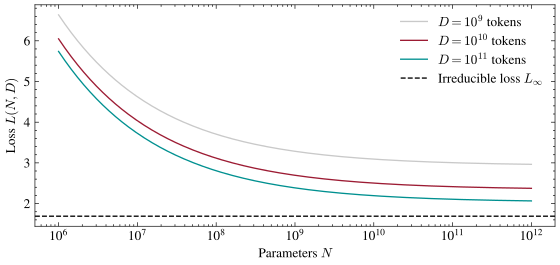
In the plot, each curve fixes a dataset size \(D\) and grows the model. The loss falls as a power law and then flattens onto the plateau \(L_\infty + B/D^{\beta}\). Past that point, reducing the loss requires more data rather than more parameters.
\(N\) and \(D\) cannot vary independently under a fixed compute budget. Training a transformer costs about \(6ND\) floating-point operations, roughly six per parameter per token (two for the forward pass and four for the backward pass), so a fixed budget \(C\) constrains their product. Any split with \(ND \propto C\) is affordable, including a large model with little data or a small model with much more data. Problem 21 supplies this model-data split under the standard compute approximation, then asks when the architecture’s sequence-length cost invalidates that approximation. The 2022 result, known as Chinchilla, showed that several models used too little training data for their parameter counts.
The transformer block still lacks position information, so the model treats “dog bites man” and “man bites dog” as the same bag of evidence. Our demo papered over this by adding a learned table of position vectors to the token embeddings. The next lecture introduces sinusoidal frequency ladders and rotations (RoPE) that make attention scores depend only on relative position. As with circulant convolution matrices, the resulting structure is Toeplitz. The causal mask, per-position MLP, and narrow heads restrict which information each computation can use. Those restrictions define much of the architecture.