Demo: Learning without an Environment Derivative

CartPole accepts a discrete action and returns a new state and reward, but its simulator supplies no derivative to the policy. We train a softmax policy with REINFORCE to see whether sampled log-probabilities provide enough of a gradient signal.

Each episode collects rewards and action log-probabilities. After the episode ends, its discounted return weights the gradient update.

import gymnasium as gym
import numpy as np
import matplotlib.pyplot as plt
import torch
import torch.nn as nn

plt.style.use("../figure_style.mplstyle")
torch.manual_seed(24)
env = gym.make("CartPole-v1")
policy = nn.Sequential(nn.Linear(4, 32), nn.ReLU(), nn.Linear(32, 2))
optimizer = torch.optim.Adam(policy.parameters(), lr=3e-3)
gamma = 0.99
n_episodes = 1200

Question: Can REINFORCE Improve a Policy through a Black-Box Environment?

The loss is the negative return times the sampled log-probability. Autodiff sees the policy computation but never env.step. Predict the moving average and decide whether individual episode returns should improve smoothly.

episode_returns = []
for episode in range(n_episodes):
    state, _ = env.reset(seed=episode)
    log_probabilities = []
    rewards = []
    done = False
    while not done:
        logits = policy(torch.tensor(state, dtype=torch.float32))
        distribution = torch.distributions.Categorical(logits=logits)
        action = distribution.sample()
        log_probabilities.append(distribution.log_prob(action))
        state, reward, terminated, truncated, _ = env.step(action.item())
        rewards.append(reward)
        done = terminated or truncated

    G = 0.0
    for t, reward in enumerate(rewards):
        G += gamma ** t * reward
    log_probability = torch.stack(log_probabilities).sum()
    loss = -G * log_probability
    optimizer.zero_grad()
    loss.backward()
    optimizer.step()
    episode_returns.append(sum(rewards))
env.close()

Returns during Training

Average each window of 50 episodes to see the trend beneath the episode-to-episode variation.

episode_returns = np.array(episode_returns)
window = 50
moving_average = []
for end in range(window, n_episodes + 1):
    moving_average.append(episode_returns[end - window:end].mean())

fig, ax = plt.subplots(figsize=(7, 3.2))
ax.plot(np.arange(1, n_episodes + 1), episode_returns, "o", markersize=2, label="Episode return")
ax.plot(np.arange(window, n_episodes + 1), moving_average, linewidth=1.7, label=f"{window}-episode moving average")
ax.set_xlabel("Episode")
ax.set_ylabel("Return (Steps Survived)")
ax.legend(frameon=False)
plt.show()

print(f"Mean return, first {window} episodes: {episode_returns[:window].mean():.1f}")
print(f"Mean return, final {window} episodes: {episode_returns[-window:].mean():.1f}")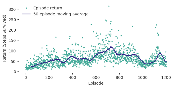

Mean return, first 50 episodes: 23.6
Mean return, final 50 episodes: 48.3

Answer. The moving average rises even though gradients never pass through the environment. The return reweights gradients of actions the policy actually sampled. Individual episodes remain jagged because actions, initial states, and trajectories are random.

REINFORCE makes black-box learning possible, but its Monte Carlo gradient is noisy. The next demo shows how a baseline can reduce that noise without changing the target gradient.