Baseline and Advantage
Last lecture REINFORCE learned CartPole from scratch, climbing from a return of \(23.7\) to \(290.5\), but its training curve lurched through progress, collapse, and recovery. One noisy scalar, the return \(G(\tau)\), multiplies the entire \(226\)-coordinate gradient. CartPole’s returns are also all positive, so no update ever pushes probability away from an action: what distinguishes a good episode from a bad one is a small difference on top of a large number they share. Problem 24 showed that shifting both of a bandit’s rewards by the same constant \(c\) leaves the true gradient unchanged while the estimator’s variance grows like \(c^2\). A control variate removes this dependence on the reward scale’s zero.
The Baseline
Recall last lecture’s estimator, written for a single episode: \[ \widehat{\nabla J} = G(\tau) \sum_{t \geq 0} \nabla_{\boldsymbol\theta} \log \pi_{\boldsymbol\theta}(a_t | s_t), \] an unbiased Monte Carlo estimate of \(\nabla_{\boldsymbol\theta} J(\boldsymbol\theta)\), the gradient of the expected return \(J(\boldsymbol\theta) = \mathbb{E}_{\tau \sim \pi_{\boldsymbol\theta}}[G(\tau)]\). Instead of weighting each episode’s score by its raw return, we propose to weight it by the return measured against a reference level \(b \in \mathbb{R}\), a scalar called a baseline: \[ \widehat{\nabla J}^{\,b} = \big(G(\tau) - b\big) \sum_{t \geq 0} \nabla_{\boldsymbol\theta} \log \pi_{\boldsymbol\theta}(a_t | s_t). \] The baseline measures each return relative to a reference level: an episode above the baseline pushes probability toward its actions, while one below it pushes away. We must check that replacing the raw return with a baselined return preserves unbiasedness.
Claim: For any baseline \(b\) that does not depend on the actions taken, \(\mathbb{E}_{\tau \sim \pi_{\boldsymbol\theta}}\left[b \, \nabla_{\boldsymbol\theta} \log p_{\boldsymbol\theta}(\tau)\right] = \mathbf{0}\), and therefore \(\mathbb{E}[\widehat{\nabla J}^{\,b}] = \nabla_{\boldsymbol\theta} J(\boldsymbol\theta)\) for every such \(b\).
Proof of Claim
The engine is a fact about the score, the gradient of the log-probability: it has mean zero under its own distribution. For any distribution \(p_{\boldsymbol\theta}\) over outcomes \(x\), the expected score vanishes: \[ \mathbb{E}_{x \sim p_{\boldsymbol\theta}}\left[\nabla_{\boldsymbol\theta} \log p_{\boldsymbol\theta}(x)\right] = \sum_x p_{\boldsymbol\theta}(x) \, \frac{\nabla_{\boldsymbol\theta} \, p_{\boldsymbol\theta}(x)}{p_{\boldsymbol\theta}(x)} = \nabla_{\boldsymbol\theta} \sum_x p_{\boldsymbol\theta}(x) = \nabla_{\boldsymbol\theta} \, 1 = \mathbf{0}, \] where we applied the log-derivative identity from last lecture, cancelled the \(p_{\boldsymbol\theta}(x)\)’s, moved the gradient outside the sum (linearity again), and used that probabilities sum to one no matter what \(\boldsymbol\theta\) is, so the gradient of that sum is the gradient of a constant. Taking \(x = \tau\), a constant baseline contributes \(b \cdot \mathbb{E}[\nabla_{\boldsymbol\theta} \log p_{\boldsymbol\theta}(\tau)] = \mathbf{0}\), and by linearity of expectation the baselined estimator has the same mean as the raw one. The same argument covers a baseline \(b(s_t)\) that varies with the state: conditioned on \(s_t\), the inner expectation \(\mathbb{E}_{a_t \sim \pi_{\boldsymbol\theta}(\cdot|s_t)}[\nabla_{\boldsymbol\theta} \log \pi_{\boldsymbol\theta}(a_t|s_t)]\) is zero at every state by the identity above, so \(\mathbb{E}[b(s_t)\, \nabla_{\boldsymbol\theta} \log \pi_{\boldsymbol\theta}(a_t|s_t)] = \mathbf{0}\) term by term.A policy cannot raise the probability of every action at once, so a baseline’s push, spread across the actions in proportion to how often the policy takes them, cancels itself exactly. Do you see where the argument breaks if \(b\) depends on the action the agent actually took?
Every action-independent \(b\) preserves unbiasedness, so we choose \(b\) to minimize variance.
A Control Variate
In the Monte Carlo lecture’s control variate section, we shrank an estimator’s variance by subtracting \(c\,(g(X) - \mathbb{E}[g])\). A surrogate quantity \(g\), correlated with the target and with a known mean, reduced variance without changing the estimator’s mean. The baseline is a control variate of exactly this form.
To see the correspondence, look at a single coordinate \(\theta\) of the parameter vector (everything applies coordinate by coordinate) and write \(u(\tau) = \frac{\partial}{\partial \theta} \log p_{\boldsymbol\theta}(\tau)\) for the score, a scalar. REINFORCE averages samples of \(f(\tau) = G(\tau)\, u(\tau)\), and the baselined version averages the control-variate adjustment of that same quantity: \[ f(\tau) - b\,\big(u(\tau) - \mathbb{E}[u(\tau)]\big), \qquad \mathbb{E}[u(\tau)] = 0. \] The surrogate is the score \(u\) itself. It is correlated with \(f = Gu\), since the two share the factor \(u\), and its mean is known exactly: it is the zero we just proved, playing the role that \(\mathbb{E}[X_1 + X_2] = 7\) played for the two dice. The baseline \(b\) is the coefficient \(c\), chosen by the same minimization used in the Monte Carlo lecture.
The Best Constant Baseline
Choose \(b\) to minimize the variance. For a single episode and a single coordinate the estimator is \(\widehat{g}_b = (G - b)\,u\), and its variance splits into a second moment minus a squared mean: \[ \textnormal{Var}(\widehat{g}_b) = \mathbb{E}\left[(G - b)^2 u^2\right] - \big(\mathbb{E}[\widehat{g}_b]\big)^2. \] The second term is the true gradient squared for every \(b\), which is exactly what unbiasedness pinned down, so only the first term responds to our choice. Expanding the square and using linearity of expectation turns that first term into a parabola in \(b\): \[ \mathbb{E}\left[(G - b)^2 u^2\right] = \mathbb{E}[G^2 u^2] - 2b\, \mathbb{E}[G u^2] + b^2\, \mathbb{E}[u^2]. \] It opens upward, because the coefficient of \(b^2\) is \(\mathbb{E}[u^2] \geq 0\). Setting its derivative \(-2\,\mathbb{E}[Gu^2] + 2b\,\mathbb{E}[u^2]\) to zero gives the bottom: \[ b^\star = \frac{\mathbb{E}[G\, u^2]}{\mathbb{E}[u^2]}. \] The optimum \(b^\star\) is a weighted average of returns, with each episode weighted by its squared score. Episodes whose probability is most sensitive to \(\theta\) receive the most weight.
The score has mean zero, so its covariance with \(Gu\) and its own variance both collapse to plain second moments: \[ \textnormal{Cov}(Gu,\, u) = \mathbb{E}[Gu \cdot u] - \mathbb{E}[Gu]\,\mathbb{E}[u] = \mathbb{E}[G u^2], \qquad \textnormal{Var}(u) = \mathbb{E}[u^2] - \big(\mathbb{E}[u]\big)^2 = \mathbb{E}[u^2]. \] Substituting both into the ratio rewrites the optimal baseline as a covariance over a variance: \[ b^\star = \frac{\textnormal{Cov}(f, g)}{\textnormal{Var}(g)} \qquad \text{with } f = Gu, \; g = u. \] This is the optimal control-variate coefficient \(c^\star = \textnormal{Cov}(f,g)/\textnormal{Var}(g)\) from Problem 2. Problem 2 also computed how much that coefficient saves: the variance drops by the factor \(1 - \rho^2\), where \(\rho\) is now the correlation between \(Gu\) and \(u\). The calculation assumes that the baseline multiplying one score is independent of that sampled action. Problem 25 tests what happens when a batch estimates its own baseline and quietly violates that condition.
The Parabola, Measured
We can measure the variance as a function of the baseline by holding a trained policy fixed and computing each episode’s gradient estimate under different values of \(b\).
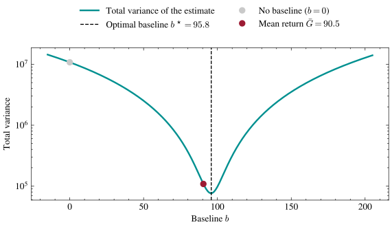
The logarithmic vertical axis shows the predicted quadratic pattern. The variance at the optimal baseline \(b^\star\) is orders of magnitude below the variance at \(b = 0\), and the mean return \(\bar{G}\) captures nearly all of that reduction.
A single constant baseline ignores differences among states.
The Advantage
The appropriate reference level depends on the state: a return of \(80\) is typical from a balanced pole but unusually high from a pole about to topple. Like par on a golf course, the baseline varies state by state.
Problem 23 defined the value function. The Q-function refines it by fixing the agent’s first action: \[ V^\pi(s) = \mathbb{E}[G_t \mid s_t = s], \qquad Q^\pi(s, a) = \mathbb{E}[G_t \mid s_t = s, \, a_t = a]. \] In words, \(V^\pi(s)\) is the expected return from state \(s\) under the current policy, and \(Q^\pi(s,a)\) fixes the first action to \(a\) and follows the policy afterward. Their difference is the advantage: \[ A^\pi(s, a) = Q^\pi(s, a) - V^\pi(s), \] how much better (or worse) action \(a\) is than the policy’s par from state \(s\). Because \(V^\pi(s) = \mathbb{E}_{a \sim \pi(\cdot|s)}[Q^\pi(s,a)]\), the advantage averages to exactly zero at every state: \[ \mathbb{E}_{a \sim \pi(\cdot|s)}\left[A^\pi(s,a)\right] = \mathbb{E}_{a \sim \pi(\cdot|s)}\left[Q^\pi(s,a)\right] - V^\pi(s) = 0. \] A positive advantage beat the policy’s own average from that state and a negative one fell short, so good and bad actions finally push in opposite directions instead of merely with different force. Practical algorithms weight each step’s score \(\nabla_{\boldsymbol\theta} \log \pi_{\boldsymbol\theta}(a_t|s_t)\) by an estimate of \(A^\pi(s_t, a_t)\), typically the observed return minus an estimate of \(V^\pi(s_t)\). (Learning \(\widehat{V}\) with a second network alongside the policy is the actor–critic family of algorithms.)
\(V^\pi(s)\) is close to, but not exactly, the variance-optimal state-dependent baseline. More importantly, the unbiasedness proof assumes that the baseline used for one sampled action does not leak information from that same action and return.
Mean-Centering Across a Batch
A common implementation runs a batch of \(N\) episodes, computes their returns \(G^{(1)}, \ldots, G^{(N)}\), and weights each episode’s score by the centered return: \[ G^{(i)} - \bar{G}, \qquad \bar{G} = \frac{1}{N} \sum_{j=1}^N G^{(j)}. \] The batch estimates its own baseline, at zero extra cost. (In practice the centered returns are usually also divided by the batch’s standard deviation, which makes the update invariant to reward scale as well as reward shift. If every episode in a batch has the same return, the standard deviation is zero, so an implementation must handle this case explicitly.) This resembles subtracting \(\mathbb{E}[G]\), but the resemblance hides a finite-batch dependence: sample \(i\) contributes to its own \(\bar G\). Problem 25 asks whether that dependence introduces bias and whether leave-one-out centering repairs it. The class demo compares raw-return and mean-centered REINFORCE updates on CartPole, including a constant shift of every reward.
Constraining the update
In reinforcement learning, an aggressive update changes both the model and the distribution of future training data. A damaged policy may stop visiting the states needed for recovery, as in last lecture’s collapse to a return of \(9\).
Trust-region methods measure update size in behavior space with the KL divergence from the Logistic Regression lecture and keep the new policy within a budget \(\delta > 0\) of the old one: \[ \mathbb{E}_s\left[\textnormal{KL}\big(\pi_{\text{old}}(\cdot|s) \,\|\, \pi_{\text{new}}(\cdot|s)\big)\right] \leq \delta. \] The constraint limits how much the policy’s behavior can change on the states it visits. PPO, proximal policy optimization, enforces the same idea more cheaply by clipping the objective once the new policy strays too far. The same constraint appears when a chatbot is fine-tuned from human feedback (RLHF), where the objective is the expected reward minus \(\beta \, \textnormal{KL}(\pi_{\boldsymbol\theta} \,\|\, \pi_{\text{ref}})\), with \(\beta > 0\) controlling the penalty and \(\pi_{\text{ref}}\) the pretrained transformer itself. The reward represents human preferences, while the KL penalty discourages the policy from moving far from the pretrained language model and exploiting weaknesses in the reward model. PPO as used in RLHF combines policy gradients, advantage-weighted updates, and a KL constraint.
The optimal policy-gradient baseline is the same control-variate coefficient derived in Problem 2. Problem 25 instead examines a practical failure mode of that theory: estimating a baseline on the same samples whose scores it multiplies, then repairing the dependence by leave-one-out. A cross-fitted learned critic is an optional extension.