Demo: Which Estimated Baselines Preserve the Gradient?

A baseline can be estimated from data, but it must not use a trajectory to define the reference multiplying that trajectory’s own score. We use a two-action policy with a known analytic gradient to test four estimators.

The setup simulates current and prior batches and computes the exact gradient for comparison.

import numpy as np
import matplotlib.pyplot as plt

plt.style.use("../figure_style.mplstyle")
rng = np.random.default_rng(25)

p = 0.35
reward_gap = 2.0
reward_offset = 10.0
noise_sd = 3.0
batch_size = 8
repetitions = 50_000
true_gradient = reward_gap * p * (1 - p)

Simulating Independent Batches

Each row is a batch. Each column is one sampled action and reward. The score for a Bernoulli action is the action minus its probability.

def draw_batches(count, size, rng):
    actions = rng.binomial(1, p, size=(count, size))
    scores = actions - p
    rewards = reward_offset + reward_gap * actions + rng.normal(
        0, noise_sd, size=(count, size)
    )
    return rewards, scores

current_rewards, current_scores = draw_batches(repetitions, batch_size, rng)
prior_rewards, _ = draw_batches(repetitions, batch_size, rng)
print(f"Analytic policy gradient: {true_gradient:.4f}")

Analytic policy gradient: 0.4550

Question 1: Which Estimated Baselines Remain Unbiased?

We compare raw REINFORCE, a baseline from an independent prior batch, the current-batch mean, and leave-one-out centering. The prior mean is random but independent of each current score. The current mean contains each trajectory’s own return.

raw = np.mean(current_rewards * current_scores, axis=1)
prior_baseline = prior_rewards.mean(axis=1, keepdims=True)
independent = np.mean((current_rewards - prior_baseline) * current_scores, axis=1)
current_mean = current_rewards.mean(axis=1, keepdims=True)
same_batch = np.mean((current_rewards - current_mean) * current_scores, axis=1)
# Remove each trajectory's own reward before averaging the others.
reward_sum = current_rewards.sum(axis=1, keepdims=True)
leave_one_out_baseline = (reward_sum - current_rewards) / (batch_size - 1)
leave_one_out = np.mean((current_rewards - leave_one_out_baseline) * current_scores, axis=1)

estimators = {
    "Raw": raw,
    "Prior-batch baseline": independent,
    "Same-batch mean": same_batch,
    "Leave one out": leave_one_out,
}
for name, values in estimators.items():
    print(f"{name:20s} mean {values.mean():.4f}, std {values.std():.4f}")
print(f"Predicted same-batch mean: {(1 - 1 / batch_size) * true_gradient:.4f}")

Raw                  mean 0.4509, std 1.9811
Prior-batch baseline mean 0.4569, std 0.5488
Same-batch mean      mean 0.3990, std 0.4865
Leave one out        mean 0.4560, std 0.5560
Predicted same-batch mean: 0.3981

The markers show estimated means, and the error bars show the spread of individual batch estimates. The horizontal lines give the exact expectations.

fig, ax = plt.subplots(figsize=(8, 3.7), layout="constrained")
names = list(estimators)
means = [estimators[name].mean() for name in names]
stds = [estimators[name].std() for name in names]
for x, mean, std in zip(range(len(names)), means, stds):
    ax.errorbar(x, mean, yerr=std, fmt="o", elinewidth=5, alpha=0.55, capsize=4, markersize=5)
ax.axhline(true_gradient, linestyle="--", linewidth=1.2,
           label="True gradient")
ax.axhline((1 - 1 / batch_size) * true_gradient, linestyle=":", linewidth=1.2, label="Same-batch expectation")
ax.set_xticks(range(len(names)))
ax.set_xticklabels(names, rotation=12, ha="right")
ax.set_ylabel("Estimator Mean and One Standard Deviation")
ax.legend(frameon=False)
plt.show()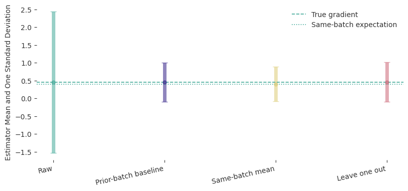

Answer. Raw REINFORCE, the independent baseline, and leave-one-out centering agree with the analytic gradient. Same-batch centering is smaller by the factor \(1-1/N\) because each return contributes to its own baseline.

Question 2: How Does the Same-Batch Bias Change with Batch Size?

We repeat the comparison for several values of \(N\). The predicted ratio is \(1-1/N\) for same-batch centering and \(1\) for leave one out.

batch_sizes = np.array([2, 4, 8, 16, 32])  # change these sizes if useful
centered_ratio = []
leave_one_out_ratio = []
for N in batch_sizes:
    rewards, scores = draw_batches(30_000, N, rng)
    current_mean = rewards.mean(axis=1, keepdims=True)
    centered = np.mean((rewards - current_mean) * scores, axis=1)
    reward_sum = rewards.sum(axis=1, keepdims=True)
    other_mean = (reward_sum - rewards) / (N - 1)
    leave_one_out = np.mean((rewards - other_mean) * scores, axis=1)
    centered_ratio.append(centered.mean() / true_gradient)
    leave_one_out_ratio.append(leave_one_out.mean() / true_gradient)

fig, ax = plt.subplots(figsize=(7, 3.1))
ax.plot(batch_sizes, centered_ratio, "o-", label="Same-batch mean")
ax.plot(batch_sizes, 1 - 1 / batch_sizes, linestyle=":",
        label="$1-1/N$")
ax.plot(batch_sizes, leave_one_out_ratio, "s-", label="Leave one out")
ax.axhline(1, linewidth=1)
ax.set_xlabel("Batch Size $N$")
ax.set_ylabel("Empirical Mean / True Gradient")
ax.set_ylim(0.45, 1.08)
ax.legend(frameon=False)
plt.show()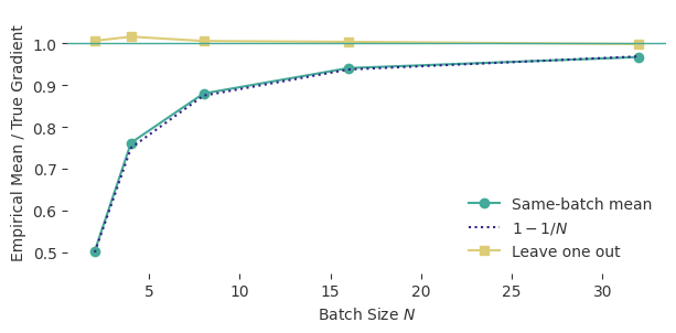

Answer. The measured ratios follow both predictions. The same-batch bias shrinks as \(N\) grows but does not vanish at finite batch size. A fixed, independent, prior-data, or leave-one-out baseline can use data without changing the gradient’s expectation.