Decompositions
Multiplying a vector by a matrix can change both its length and its direction. Some directions are easier to track: an eigenvector stays on the same line after multiplication. Eigenvalues and singular values describe how much a matrix stretches these directions, which will help us solve linear systems and compress data.
Eigenvectors
In the previous reading, we described a matrix by how its rows combine input coordinates. That description is useful for computing an output, but it can hide the geometry: a matrix may mix the standard coordinates even when it stretches along other axes. To find those axes, we look for a nonzero vector whose output stays on the same line. For a square matrix \(\mathbf A\in\mathbb R^{d\times d}\), such an eigenvector \(\mathbf v\) satisfies \[ \mathbf A\mathbf v=\lambda\mathbf v. \] The corresponding eigenvalue \(\lambda\) records what the map does along that direction. For a real eigenvalue, its magnitude gives the stretch, and its sign determines whether the direction reverses. A zero eigenvalue means the direction is erased.
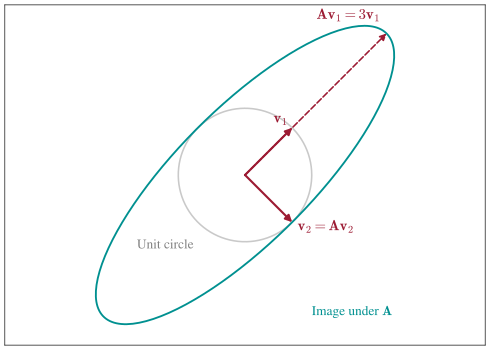
In the figure, the eigenvectors become the axes of the ellipse. Every input is a combination of these two perpendicular directions, so knowing the stretch along each one tells us the entire action of the matrix.
The spectral theorem guarantees this structure for every real symmetric matrix, meaning \(\mathbf A^\top=\mathbf A\). It says that we can choose \(d\) real eigenvectors \(\mathbf v_1,\ldots,\mathbf v_d\) that form an orthonormal basis: they have length one, are pairwise perpendicular, and span \(\mathbb R^d\). Let \(\lambda_i\) be the eigenvalue corresponding to \(\mathbf v_i\), for \(i=1,\ldots,d\). Thus \(\mathbf v_i^{\top}\mathbf v_j\) is one when \(i=j\) and zero otherwise, and every input has the expansion \[ \mathbf x=\sum_{i=1}^d(\mathbf v_i^{\top}\mathbf x)\mathbf v_i. \] This is what makes the eigenvectors useful as coordinates: the inner product \(\mathbf v_i^{\top}\mathbf x\) measures how much of the input lies along the \(i\)th direction.
Why does an orthonormal eigenbasis exist?
We first find one eigenvector, then show that we can search for the others in the space perpendicular to it. For a unit vector \(\mathbf v\), the quantity \(\mathbf v^\top\mathbf A\mathbf v\) measures the component of its output along its input direction. Choose a unit vector \(\mathbf v\) that maximizes this quantity. A maximizer exists because a continuous function attains a maximum on the unit sphere, which is closed and bounded.
At a maximum, a small change of direction cannot increase this quantity to first order. To express that with a one-variable derivative, take any \(\mathbf w\) perpendicular to \(\mathbf v\) and normalize \(\mathbf v+t\mathbf w\) to keep it on the unit sphere. The value along this curve is \[ g(t)=\frac{(\mathbf v+t\mathbf w)^\top\mathbf A(\mathbf v+t\mathbf w)} {1+t^2\|\mathbf w\|_2^2}. \] Since \(t=0\) is a maximum and \(\mathbf A\) is symmetric, \[ 0=g'(0) =\mathbf w^\top\mathbf A\mathbf v+\mathbf v^\top\mathbf A\mathbf w =2\mathbf w^\top\mathbf A\mathbf v. \] So \(\mathbf A\mathbf v\) is perpendicular to every vector perpendicular to \(\mathbf v\). It must lie along \(\mathbf v\), giving \(\mathbf A\mathbf v=\lambda\mathbf v\) for a real scalar \(\lambda\).
Now symmetry ensures that a vector \(\mathbf w\) perpendicular to \(\mathbf v\) stays perpendicular after applying \(\mathbf A\): \[ \mathbf v^\top\mathbf A\mathbf w =(\mathbf A\mathbf v)^\top\mathbf w =\lambda\mathbf v^\top\mathbf w =0. \] The restriction of \(\mathbf A\) to this \((d-1)\)-dimensional space is therefore a symmetric map from that space to itself. Repeat the same argument there to find a second unit eigenvector, perpendicular to the first. Continuing in the remaining perpendicular space produces \(d\) mutually perpendicular unit eigenvectors. In one dimension, every linear map is scalar multiplication. These vectors form the required orthonormal eigenbasis.
Once we have this basis, the matrix formula follows by checking its action on each eigenvector. Set \(\mathbf B=\sum_{i=1}^d\lambda_i\mathbf v_i\mathbf v_i^{\top}\). Orthonormality gives \[ \mathbf B\mathbf v_j =\sum_{i=1}^d\lambda_i\mathbf v_i(\mathbf v_i^{\top}\mathbf v_j) =\lambda_j\mathbf v_j =\mathbf A\mathbf v_j. \] Since \(\mathbf A\) and \(\mathbf B\) agree on a basis, they agree on every input and are the same matrix. Putting the eigenvectors in the columns of \(\mathbf V\) and their eigenvalues on the diagonal of \(\boldsymbol\Lambda\) gives the two equivalent forms \[ \mathbf A =\mathbf V\boldsymbol\Lambda\mathbf V^\top =\sum_{i=1}^d\lambda_i\mathbf v_i\mathbf v_i^{\top}. \] Read the factorization from right to left: \(\mathbf V^\top\) computes the eigenvector coordinates, \(\boldsymbol\Lambda\) scales them, and \(\mathbf V\) combines the scaled directions into the output. The outer-product form uses the multiplication rule from the previous reading. Each term \(\lambda_i\mathbf v_i\mathbf v_i^{\top}\) keeps only the input component along \(\mathbf v_i\) and scales it by \(\lambda_i\).
Inverting a Symmetric Matrix
The inverse must undo each eigenvalue’s scaling, so it scales the same direction by the reciprocal eigenvalue.
Claim: A real symmetric matrix \(\mathbf A\) is invertible exactly when all its eigenvalues are nonzero. In that case, its orthonormal eigenvectors give \[ \mathbf A^{-1} =\sum_{i=1}^d\frac{1}{\lambda_i}\mathbf v_i\mathbf v_i^{\top} =\mathbf V\boldsymbol\Lambda^{-1}\mathbf V^\top. \]
Proof
If \(\lambda_j=0\), then \(\mathbf A\mathbf v_j=\mathbf0\) for a nonzero vector \(\mathbf v_j\), so \(\mathbf A\) cannot be invertible. Otherwise, set \(\mathbf B=\sum_{i=1}^d(\lambda_i)^{-1}\mathbf v_i\mathbf v_i^{\top}\). Orthonormality gives \(\mathbf B\mathbf v_j=\lambda_j^{-1}\mathbf v_j\) for \(j=1,\ldots,d\). Each composition therefore undoes the scaling on every eigenvector: \[ \begin{aligned} \mathbf A\mathbf B\mathbf v_j&=\lambda_j^{-1}\mathbf A\mathbf v_j=\mathbf v_j,\\ \mathbf B\mathbf A\mathbf v_j&=\lambda_j\mathbf B\mathbf v_j=\mathbf v_j. \end{aligned} \] Both products agree with \(\mathbf I\) on a basis, so \(\mathbf A\mathbf B=\mathbf B\mathbf A=\mathbf I\). Thus \(\mathbf B=\mathbf A^{-1}\).
The Power Method
We still need to find the eigenvectors promised by the spectral theorem. Matrix powers give us a way to isolate a leading direction.
Claim: For a symmetric matrix \(\mathbf A\) with orthonormal eigenvectors \(\mathbf v_i\) and eigenvalues \(\lambda_i\), every integer \(k\geq1\) satisfies \[ \mathbf A^k=\sum_{i=1}^d\mathbf v_i\lambda_i^k\mathbf v_i^{\top}. \]
Proof
Each multiplication by \(\mathbf A\) scales \(\mathbf v_i\) by \(\lambda_i\), so \(\mathbf A^k\mathbf v_i=\lambda_i^k\mathbf v_i\) for \(i=1,\ldots,d\). Apply this to the eigenbasis expansion of any \(\mathbf x\in\mathbb R^d\): \[ \begin{aligned} \mathbf A^k\mathbf x &=\sum_{i=1}^d(\mathbf v_i^\top\mathbf x)\lambda_i^k\mathbf v_i\\ &=\left(\sum_{i=1}^d\mathbf v_i\lambda_i^k\mathbf v_i^\top\right)\mathbf x. \end{aligned} \] The two matrices agree on every input, proving the formula.
For \(d\geq2\), write a unit starting vector as \(\mathbf q^{(0)}=\sum_{i=1}^d c_i\mathbf v_i\), where \(c_i=\mathbf v_i^\top\mathbf q^{(0)}\) for \(i=1,\ldots,d\). Assume \(c_1\ne0\) and \(|\lambda_1|>|\lambda_2|\geq\cdots\geq|\lambda_d|\). The power formula separates the leading direction from the remaining components: \[ \begin{aligned} \mathbf A^k\mathbf q^{(0)}&=c_1\lambda_1^k(\mathbf v_1+\mathbf r^{(k)}),\\ \mathbf r^{(k)}&=\sum_{i=2}^d\frac{c_i}{c_1} \left(\frac{\lambda_i}{\lambda_1}\right)^k\mathbf v_i. \end{aligned} \] Every ratio has magnitude less than one, so \(\mathbf r^{(k)}\) approaches zero. Repeated multiplication therefore reveals \(\mathbf v_1\), up to scale and sign. The power method controls the length by normalizing after each multiplication: \[ \mathbf q^{(k)} =\frac{\mathbf A\mathbf q^{(k-1)}} {\|\mathbf A\mathbf q^{(k-1)}\|_2}. \] Normalization preserves the direction of \(\mathbf A^k\mathbf q^{(0)}\). To compute the distance to \(\mathbf v_1\), first assume \(\lambda_1>0\) and choose the sign of \(\mathbf v_1\) so that \(c_1>0\).
Claim: Under these assumptions, after \(k\geq1\) power-method steps, \[ \|\mathbf v_1-\mathbf q^{(k)}\|_2 \leq \frac{\sqrt{\sum_{i=2}^d c_i^2}}{c_1} \left|\frac{\lambda_2}{\lambda_1}\right|^k. \]
Proof
Orthonormality gives the squared length of the remaining components: \[ \begin{aligned} (\delta^{(k)})^{2}:=\|\mathbf r^{(k)}\|_2^2 &=\sum_{i=2}^d\frac{c_i^2}{c_1^2} \left(\frac{\lambda_i}{\lambda_1}\right)^{2k}\\ &\leq\frac{\sum_{i=2}^d c_i^2}{c_1^2} \left|\frac{\lambda_2}{\lambda_1}\right|^{2k}. \end{aligned} \] Since \(\mathbf r^{(k)}\perp\mathbf v_1\), normalizing cancels the positive scale \(c_1\lambda_1^k\) and gives \[ \mathbf q^{(k)}=\frac{\mathbf v_1+\mathbf r^{(k)}}{\sqrt{1+(\delta^{(k)})^{2}}}. \] Since \(\mathbf v_1\) and \(\mathbf q^{(k)}\) have length one, their exact squared distance is \[ \begin{aligned} \|\mathbf v_1-\mathbf q^{(k)}\|_2^2 &=2-2\mathbf v_1^{\top}\mathbf q^{(k)}\\ &=2-\frac{2}{\sqrt{1+(\delta^{(k)})^{2}}}\\ &=\frac{2(\delta^{(k)})^{2}} {\sqrt{1+(\delta^{(k)})^{2}}\bigl(\sqrt{1+(\delta^{(k)})^{2}}+1\bigr)} \leq(\delta^{(k)})^{2}. \end{aligned} \] The last denominator is at least \(2\). Taking square roots gives \(\|\mathbf v_1-\mathbf q^{(k)}\|_2\leq\delta^{(k)}\) and proves the bound.
If \(\lambda_1<0\), the iterates alternate sign. The same bound applies with target \((-1)^k\mathbf v_1\).
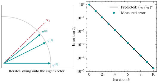
The figure plots \(\delta^{(k)}\), which also bounds the vector error after accounting for sign. Convergence is slow when \(|\lambda_2/\lambda_1|\) is near one, and a start with \(c_1=0\) cannot recover the leading direction.
Opinion dynamics. People often adjust their opinions toward those of their friends. In DeGroot learning, we model this by repeatedly averaging opinions across a friendship network. One round is a matrix multiplication, so repeated averaging uses the same mechanism as the power method. Under suitable assumptions, opinions approach a constant vector: everyone agrees.
But we can also subtract the average and rescale to see who remains above or below it. This removes the all-ones direction and brings another eigenvector into view. Problem 4 asks you to build the averaging matrix and determine how much this remaining pattern depends on the starting opinions. The connection to political polarization is about the formation of opposing groups relative to the average, even while the absolute differences shrink.
The Singular Value Decomposition
Our original question about stretch also makes sense for a rectangular matrix, such as a map from \(d\) input features to \(n\) outputs. But the equation \(\mathbf A\mathbf v=\lambda\mathbf v\) requires the input and output to live in the same space. Even for a square matrix, an orthonormal eigenbasis is not guaranteed without symmetry. To handle any matrix, we allow an input direction \(\mathbf v_i\) to map to a different output direction \(\mathbf u_i\). The singular value decomposition (SVD) chooses orthonormal directions on each side so that the map again acts on one coordinate at a time.
For \(\mathbf A\in\mathbb R^{n\times d}\), the column space is its set of possible outputs: \[ \operatorname{col}(\mathbf A) =\{\mathbf A\mathbf x:\mathbf x\in\mathbb R^d\}. \] Its dimension is the rank of \(\mathbf A\). If this dimension is \(r\), only \(r\) independent output directions are needed to describe everything the matrix can produce. That is why the decomposition below has \(r\) terms.
Claim: Every matrix \(\mathbf A\in\mathbb R^{n\times d}\) has a decomposition \[ \mathbf A =\mathbf U\boldsymbol\Sigma\mathbf V^\top =\sum_{i=1}^r\sigma_i\mathbf u_i\mathbf v_i^{\top}, \] where \(r=\operatorname{rank}(\mathbf A)\), \(\mathbf U\in\mathbb R^{n\times r}\) and \(\mathbf V\in\mathbb R^{d\times r}\) have orthonormal columns, and \(\boldsymbol\Sigma=\operatorname{diag}(\sigma_1,\ldots,\sigma_r)\) with \(\sigma_1\geq\cdots\geq\sigma_r>0\) when \(r>0\). Each right singular vector maps to its left partner: \[ \mathbf A\mathbf v_i=\sigma_i\mathbf u_i. \]
An empty sum is zero, so the outer-product formula also covers the zero matrix, whose rank is \(r=0\). The positive numbers \(\sigma_i\) are the singular values: each gives the output length for the corresponding unit input \(\mathbf v_i\). As in the eigenvector factorization, \(\mathbf V^\top\mathbf x\) computes input coordinates and \(\boldsymbol\Sigma\) scales them. The change is that \(\mathbf U\) uses a separate set of output directions, which can live in a space of a different dimension. For the rank-two \(2\times3\) matrix in the figure, two perpendicular input directions survive and the third is mapped to zero.

To find these directions, we need a way to measure stretch while working entirely in the input space. The identity \(\|\mathbf A\mathbf x\|_2^2=\mathbf x^\top(\mathbf A^\top\mathbf A)\mathbf x\) supplies it: the square, symmetric matrix \(\mathbf A^\top\mathbf A\) records the squared output length for every input. We can apply the spectral theorem to this matrix, then use \(\mathbf A\) to find the matching output directions.
Proof
The matrix \(\mathbf A^\top\mathbf A\in\mathbb R^{d\times d}\) is symmetric, so the spectral theorem gives it an orthonormal eigenbasis \(\mathbf v_1,\ldots,\mathbf v_d\). Its eigenvalues are nonnegative: for a unit eigenvector \(\mathbf v_i\) with eigenvalue \(\mu_i\), \[ \mu_i =\mathbf v_i^{\top}\mathbf A^\top\mathbf A\mathbf v_i =\|\mathbf A\mathbf v_i\|_2^2 \geq0. \] This also tells us that the stretch along \(\mathbf v_i\) is the square root of its eigenvalue. If every eigenvalue is zero, \(\mathbf A\) maps every basis vector to zero, so \(\mathbf A=\mathbf0\) and the empty sum gives its SVD. Otherwise, there is at least one positive eigenvalue. Write the \(q\) positive eigenvalues as \[ \sigma_1^2\geq\cdots\geq\sigma_q^2>0 \] and normalize each nonzero output to define its direction: \[ \mathbf u_i=\frac{\mathbf A\mathbf v_i}{\sigma_i} \qquad\text{for }i=1,\ldots,q. \] Dividing by \(\sigma_i=\|\mathbf A\mathbf v_i\|_2\) makes each \(\mathbf u_i\) a unit vector and gives \(\mathbf A\mathbf v_i=\sigma_i\mathbf u_i\). We also need the output directions to be perpendicular. Otherwise their contributions to output length would mix. Their inner products are \[ \begin{aligned} \mathbf u_i^{\top}\mathbf u_j &=\frac{\mathbf v_i^{\top}\mathbf A^\top\mathbf A\mathbf v_j} {\sigma_i\sigma_j}\\ &=\frac{\sigma_j^2}{\sigma_i\sigma_j} \mathbf v_i^{\top}\mathbf v_j, \end{aligned} \] which is one when \(i=j\) and zero otherwise.
We have described the action on every eigenvector with a positive eigenvalue. The remaining eigenvectors contribute no output, because a zero eigenvalue gives \[ \|\mathbf A\mathbf v_i\|_2^2 =\mathbf v_i^{\top}\mathbf A^\top\mathbf A\mathbf v_i =0, \] so \(\mathbf A\mathbf v_i=\mathbf0\). Now expand any input \(\mathbf x\) in the full eigenbasis and apply \(\mathbf A\). The zero-eigenvalue terms disappear, leaving \[ \begin{aligned} \mathbf A\mathbf x &=\sum_{i=1}^q (\mathbf v_i^{\top}\mathbf x)\mathbf A\mathbf v_i\\ &=\sum_{i=1}^q \sigma_i\mathbf u_i\mathbf v_i^{\top}\mathbf x. \end{aligned} \] Thus \(\mathbf A\) equals the claimed outer-product sum, and collecting its vectors into columns gives \(\mathbf U\boldsymbol\Sigma\mathbf V^\top\). To check the number of terms, the last display puts every output in the span of \(\mathbf u_1,\ldots,\mathbf u_q\). Conversely, each \(\mathbf u_i=\mathbf A(\mathbf v_i/\sigma_i)\) is itself an output. These orthonormal vectors therefore form a basis of the column space, so \(q=\operatorname{rank}(\mathbf A)=r\). This proves both forms of the SVD.
We can now answer the question about greatest stretch for any nonzero matrix. The largest singular value \(\sigma_1\) is attained by the unit input \(\mathbf v_1\). To show it is the greatest stretch, we must check that mixing input directions cannot produce a longer output. Using the full right eigenbasis from the proof, write a unit vector as \(\mathbf x=\sum_{i=1}^d c_i\mathbf v_i\), where \(c_i=\mathbf v_i^\top\mathbf x\) for \(i=1,\ldots,d\) and \(\sum_{i=1}^d c_i^2=1\). Its image is \[ \mathbf A\mathbf x =\sum_{i=1}^r \sigma_i c_i\mathbf u_i. \] The perpendicular output directions let us add squared lengths without cross terms. Since every \(\sigma_i\leq\sigma_1\), we get \[ \begin{aligned} \|\mathbf A\mathbf x\|_2^2 &=\sum_{i=1}^r\sigma_i^2c_i^2\\ &\leq\sigma_1^2\sum_{i=1}^r c_i^2\\ &\leq\sigma_1^2\sum_{i=1}^d c_i^2\\ &=\sigma_1^2. \end{aligned} \] Equality holds at \(\mathbf x=\mathbf v_1\), so \(\sigma_1\) is the greatest stretch. For the zero matrix, every input is erased and the greatest stretch is zero.
The SVD orders input directions by how much they contribute to the output per unit input length. Keeping the terms with large singular values and dropping those with small ones gives a way to approximate a matrix with fewer directions, which we will develop in low-rank approximation. The same factorization also makes it possible to store a compact change to a neural network’s weights, an application called low-rank adaptation (LoRA). Eigenvalue magnitudes control repeated multiplication, and singular values identify the directions of greatest stretch.