Gradient Descent
Solving the least-squares equations can be expensive when there are many features. Gradient descent takes a different approach: start with a guess and repeatedly adjust the weights to reduce the loss. The step size and the units of the features can make this process converge quickly, crawl, or diverge.
Repeating the Update
Keep the design matrix \(\mathbf X\in\mathbb R^{n\times d}\) for \(n\geq1\) training examples with \(d\) features, labels \(\mathbf y\in\mathbb R^n\), and weights \(\mathbf w\in\mathbb R^d\). The least-squares reading derived the mean squared error gradient: \[ \nabla\mathcal{L}(\mathbf w)=-\frac2n\mathbf X^\top(\mathbf y-\mathbf X\mathbf w). \] Setting it to zero gives the normal equations. We can also use it to improve the weights one step at a time.
Gradient descent adjusts all weights using their derivatives. Starting from randomly initialized weights \(\mathbf w^{(0)}\), it repeats \[ \begin{aligned} \mathbf w^{(t+1)} =\mathbf w^{(t)}-\alpha\nabla\mathcal{L}(\mathbf w^{(t)}) \end{aligned} \] where \(t\) counts updates and \(\alpha>0\) is the learning rate. To see why we subtract the gradient, use the first-order approximation for a small change \(\Delta\mathbf w\in\mathbb R^d\): \[ \mathcal{L}(\mathbf w+\Delta\mathbf w) \approx\mathcal{L}(\mathbf w)+\nabla\mathcal{L}(\mathbf w)^\top\Delta\mathbf w. \] Substituting \(\Delta\mathbf w=-\alpha\nabla\mathcal{L}(\mathbf w)\) gives \[ \begin{aligned} \mathcal{L}\bigl(\mathbf w-\alpha\nabla\mathcal{L}(\mathbf w)\bigr) &\approx\mathcal{L}(\mathbf w)-\alpha\nabla\mathcal{L}(\mathbf w)^\top\nabla\mathcal{L}(\mathbf w)\\ &=\mathcal{L}(\mathbf w)-\alpha\|\nabla\mathcal{L}(\mathbf w)\|_2^2. \end{aligned} \] When the gradient is nonzero, the approximation predicts a decrease. For sufficiently small positive \(\alpha\), the actual loss decreases too. The learning rate controls how far we move. A large step can overshoot because the first-order approximation is only local. We measure progress by the distance to the minimizing weights, relative to the starting distance.
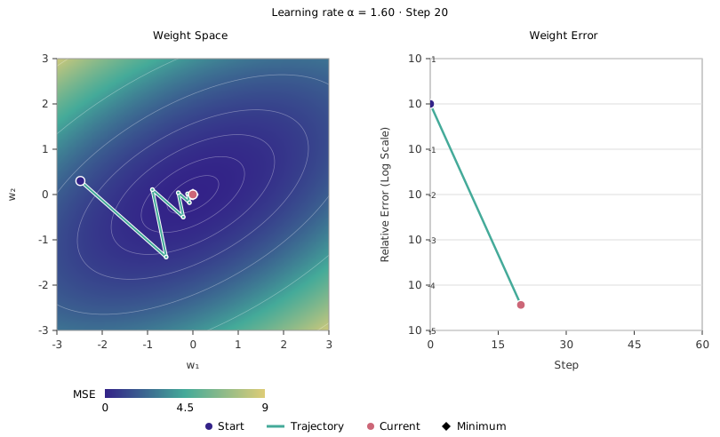
Weight Space
Weight Error
Each update uses two matrix-vector products, costing \(O(nd)\) for a dense design matrix. After \(T\) updates, the cost is \(O(Tnd)\), compared with \(O(nd^2+d^3)\) to build and solve the normal equations when the columns are independent. Gradient descent is useful when sufficiently few of these cheap updates reach the desired accuracy.
To track progress, compare the current weights with a least-squares solution \(\mathbf w^\star\). The error in the weights is \[ \mathbf e^{(t)}=\mathbf w^{(t)}-\mathbf w^\star. \] The loss’s Hessian, the matrix of second partial derivatives, is \[ \mathbf H=\frac2n\mathbf X^\top\mathbf X\in\mathbb R^{d\times d}. \] It describes how quickly the gradient changes as we move the weights.
Claim: Gradient descent updates the weight error by the same matrix at every step: \[ \mathbf e^{(t+1)}=(\mathbf I-\alpha\mathbf H)\mathbf e^{(t)}, \qquad \mathbf e^{(t)}=(\mathbf I-\alpha\mathbf H)^t\mathbf e^{(0)}. \] The loss above the minimum is \[ \mathcal{L}(\mathbf w^{(t)})-\mathcal{L}(\mathbf w^\star) =\frac1n\|\mathbf X\mathbf e^{(t)}\|_2^2. \]
Proof
The normal equations from the previous reading give \(\mathbf X^\top\mathbf y=\mathbf X^\top\mathbf X\mathbf w^\star\). Use them to express the gradient in terms of the weight error: \[ \begin{aligned} \nabla\mathcal L(\mathbf w^{(t)}) &=\frac2n\mathbf X^\top\mathbf X(\mathbf w^{(t)}-\mathbf w^\star)\\ &=\mathbf H\mathbf e^{(t)}. \end{aligned} \] Subtracting \(\mathbf w^\star\) from the update therefore gives \[ \begin{aligned} \mathbf e^{(t+1)} &=\mathbf w^{(t)}-\alpha\mathbf H\mathbf e^{(t)}-\mathbf w^\star\\ &=(\mathbf I-\alpha\mathbf H)\mathbf e^{(t)}. \end{aligned} \] Applying this recurrence \(t\) times gives \[ \mathbf e^{(t)}=(\mathbf I-\alpha\mathbf H)^t\mathbf e^{(0)}. \]
The least-squares reading also established that adding a weight change \(\mathbf h\) to a minimizer increases its loss by \(\|\mathbf X\mathbf h\|_2^2/n\). The cross term vanishes because the fitted residual is perpendicular to every reachable prediction change, though it need not be perpendicular to \(\mathbf y\). Applying that identity with \(\mathbf h=\mathbf e^{(t)}\) gives \[ \mathcal{L}(\mathbf w^{(t)})-\mathcal{L}(\mathbf w^\star) =\frac1n\|\mathbf X\mathbf e^{(t)}\|_2^2. \]
Thus shrinking the weight error to zero also brings the loss to its minimum. We can use the matrix-power argument from the decompositions reading to decide whether this error shrinks.
When the Error Shrinks
Assume here that the feature columns are independent, so the least-squares weights are unique. The symmetric matrix \(\mathbf H\) has an orthonormal eigenbasis \(\mathbf v_1,\ldots,\mathbf v_d\). Its eigenvalues are positive: for each unit eigenvector, \[ \lambda_i=\mathbf v_i^{\top}\mathbf H\mathbf v_i =\frac2n\|\mathbf X\mathbf v_i\|_2^2>0. \] Write the smallest and largest eigenvalues as \(\lambda_{\min}\) and \(\lambda_{\max}\).
Along each eigenvector, the update matrix acts by a scalar: \[ (\mathbf I-\alpha\mathbf H)\mathbf v_i =(1-\alpha\lambda_i)\mathbf v_i. \] Every step multiplies the error component in that direction by \(1-\alpha\lambda_i\). An absolute value below one shrinks the component. A negative factor also reverses its sign. An absolute value above one makes a nonzero component grow.
Claim: With independent feature columns, gradient descent converges to the least-squares solution \(\mathbf w^\star\) from every starting vector exactly when \[ 0<\alpha<\frac2{\lambda_{\max}}. \]
Proof
Apply the eigenvector formula for matrix powers from the decompositions reading: \[ \begin{aligned} \mathbf e^{(t)} &=(\mathbf I-\alpha\mathbf H)^t\mathbf e^{(0)}\\ &=\sum_{i=1}^d(1-\alpha\lambda_i)^t \mathbf v_i\mathbf v_i^{\top}\mathbf e^{(0)}. \end{aligned} \] Every term tends to zero if \(|1-\alpha\lambda_i|<1\) for all \(i\). Conversely, if any factor has magnitude at least one, starting with \(\mathbf e^{(0)}=\mathbf v_i\) gives an error that does not approach zero. Since each \(\lambda_i>0\), the required inequalities are \[ -1<1-\alpha\lambda_i<1 \quad\Longleftrightarrow\quad 0<\alpha<\frac2{\lambda_i}. \] They hold for every direction exactly when \(0<\alpha<2/\lambda_{\max}\).
The eigenvalues measure curvature: how quickly the gradient changes along each direction. The largest curvature limits the learning rate. If another curvature is much smaller, a rate that is safe for the steep direction barely changes the error in the shallow direction. Increasing the rate to accelerate that slow direction can make the steep direction oscillate or diverge.
The spread in curvatures is measured by the condition number of the Hessian: \[ \kappa=\frac{\lambda_{\max}}{\lambda_{\min}}. \] For least squares, this equals the squared ratio of the largest and smallest singular values of \(\mathbf X\), because the eigenvalues of \(\mathbf X^\top\mathbf X\) are the squared singular values. We can quantify how this spread limits even the best fixed learning rate.
Choosing a Fixed Learning Rate
Claim: The fixed learning rate \[ \alpha=\frac2{\lambda_{\max}+\lambda_{\min}} \] minimizes the largest absolute error multiplier across all eigendirections. That worst-direction contraction factor is \[ \max_i|1-\alpha\lambda_i|=\frac{\kappa-1}{\kappa+1}. \]
Proof
As \(\lambda_i\) ranges between the smallest and largest eigenvalues, \(1-\alpha\lambda_i\) lies between their two endpoint values. Its absolute value cannot exceed the larger endpoint magnitude, so \[ \max_i|1-\alpha\lambda_i| =\max\bigl\{|1-\alpha\lambda_{\min}|,\ |1-\alpha\lambda_{\max}|\bigr\}. \] Balance the endpoint values with opposite signs: \[ 1-\alpha\lambda_{\min}=-(1-\alpha\lambda_{\max}) \quad\Longrightarrow\quad \alpha=\frac2{\lambda_{\max}+\lambda_{\min}}. \] At this rate, both magnitudes equal \[ \frac{\lambda_{\max}-\lambda_{\min}} {\lambda_{\max}+\lambda_{\min}} =\frac{\kappa-1}{\kappa+1}. \] A smaller rate makes \(1-\alpha\lambda_{\min}\) larger than this value. A larger rate makes \(\alpha\lambda_{\max}-1\) larger than this value. Thus every other rate has a larger worst-direction factor.
When \(\kappa\) is large, this factor is close to one: even the best fixed learning rate leaves some errors shrinking slowly.
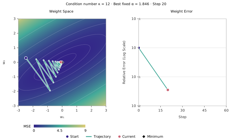
Weight Space
Weight Error
If the feature columns are dependent, \(\mathbf H\) has zero eigenvalues and its condition number is infinite. An error component in a zero-eigenvalue direction is multiplied by one, so the updates leave it unchanged. The other components can still shrink, producing a least-squares fit whose weights need not be the minimum-norm choice.
Feature Scaling
Poor conditioning can come from features measured on very different scales. Changing units changes the sizes of the feature columns and the loss’s curvatures. We can make that change while preserving the model’s possible predictions.
For feature scaling, divide column \(j\) by a positive scale \(s_j\) and multiply its weight \(w_j\) by the same scale. The contribution of every column stays the same: \[ \sum_{j=1}^d\frac{[\mathbf X]_{:,j}}{s_j}(s_jw_j) =\sum_{j=1}^d[\mathbf X]_{:,j}w_j =\mathbf X\mathbf w. \] Because every \(s_j\) is nonzero, dividing the scaled weights by their scales reverses this correspondence. Thus the scaled and original features generate exactly the same prediction vectors and have the same minimum training MSE.
Scaling changes how gradient descent moves through those predictions. Balancing the feature scales can bring the curvatures closer together, allowing one learning rate to make useful progress in more directions.
Changing units cannot turn exactly dependent columns into independent ones. Nearly parallel columns can also remain poorly conditioned after scaling: they still provide very similar information. Problem 7 asks how much scaling can help when two feature columns point in nearly the same direction.
With a safe learning rate, gradient descent reaches a least-squares fit by repeatedly shrinking its error. The largest curvature limits the step size. The spread in curvatures controls how quickly all directions improve.