Model Evaluation
A model can fit its training data well and still make poor predictions. We want its average error on new examples from the population, which we estimate using an independent sample.
Population Error and Empirical Error
Let \(P\) be the joint probability distribution of the examples we want to predict. Writing \((X,Y)\sim P\) means that the feature vector \(X\in\mathbb R^d\) and numerical label \(Y\in\mathbb R\) are drawn from this distribution, where \(d\) is the number of features. A model class \(\mathcal F\) is a set of candidate prediction rules \(f:\mathbb R^d\to\mathbb R\). For a fixed model \(f\in\mathcal F\), our target is its population error (also called risk): \[ R(f)=\mathbb E_{(X,Y)\sim P}\left[(Y-f(X))^2\right]. \] We cannot calculate this expectation directly because we do not know \(P\). Given an evaluation sample \(S=\bigl((\mathbf x_i,y_i)\bigr)_{i=1}^m\) of \(m\) independent examples from \(P\), we use the empirical error: \[ \widehat R_S(f) =\frac1m\sum_{i=1}^m\bigl(y_i-f(\mathbf x_i)\bigr)^2. \] Here \(\mathbf x_i\in\mathbb R^d\) and \(y_i\in\mathbb R\) are the features and label of example \(i\). The bold symbol \(\mathbf x_i\) denotes the entire feature vector of example \(i\). Applying our Monte Carlo sample-mean calculation to the single-example loss \(\ell=(Y-f(X))^2\): \[ \mathbb E_S[\widehat R_S(f)]=R(f), \qquad \operatorname{Var}_S(\widehat R_S(f)) =\frac{\operatorname{Var}(\ell)}m. \] The subscripts \(S\) mean that we average over repeated draws of the evaluation sample. \(f\) stays fixed. The expectation identity assumes finite expected loss, and the variance formula assumes \(\ell\) has finite variance. More evaluation examples make the estimate less noisy.
These formulas assume that \(f\) is fixed before we draw \(S\). A fitted model \(\hat f\) depends on its training examples. Let \(\widehat R_{\mathrm{train}}(f)\) be the empirical error computed on the training set. Empirical risk minimization chooses a model with the smallest training error in \(\mathcal F\): \[ \hat f\in\arg\min_{f\in\mathcal F}\widehat R_{\mathrm{train}}(f). \] Here \(\arg\min\) denotes the set of minimizing models. Assume a minimum is attained. Minimizing error on these examples makes training error optimistic on average. We evaluate \(\hat f\) on a separate sample that did not influence the fit.
| Data | Used to choose or measure |
|---|---|
| Training | Weights, such as the least-squares coefficients |
| Validation | Model choices, such as which features to include |
| Test | Error of the final model, after all choices are finished |
For example, fit a line and a quadratic on the training set, choose between them using validation error, then report the winner’s test error. Once we use validation scores to choose a model, the winning score may be optimistic too. Repeatedly changing a model after seeing test scores creates the same problem.
Adding Features to the Model
Consider polynomial regression with one scalar input \(x\in\mathbb R\) and a nonnegative integer degree \(k\). The degree-\(k\) model class is the set of all prediction rules we can obtain by choosing their coefficients: \[ \mathcal F_k =\left\{x\mapsto w_0+w_1x+\cdots+w_kx^k: \mathbf w\in\mathbb R^{k+1}\right\}. \] The weight vector \(\mathbf w=(w_0,\ldots,w_k)^\top\) contains the polynomial coefficients, so its subscripts identify coordinates, while \(x^k\) is an ordinary power. These classes are nested, meaning \(\mathcal F_k\subseteq\mathcal F_{k+1}\): setting the last coefficient to zero recovers any model in \(\mathcal F_k\).
For \(n\) training examples \((x_i,y_i)\), collect the labels into \(\mathbf y=(y_1,\ldots,y_n)^\top\in\mathbb R^n\). Increasing the degree adds a column to the design matrix \(\mathbf X_k\in\mathbb R^{n\times(k+1)}\): \[ \mathbf X_k= \begin{bmatrix} 1&x_1&\cdots&x_1^k\\ \vdots&\vdots&&\vdots\\ 1&x_n&\cdots&x_n^k \end{bmatrix}, \qquad \mathbf X_{k+1}=[\,\mathbf X_k\mid\mathbf z\,], \quad z_i=x_i^{k+1}. \] Here \(\mathbf z\in\mathbb R^n\) is the new feature column, with coordinate \(z_i\) for example \(i\). The subscript on \(\mathbf X_k\) records the degree. The larger model can reproduce every prediction of the smaller one: \[ \mathbf X_{k+1} \begin{bmatrix}\mathbf w\\0\end{bmatrix} =\mathbf X_k\mathbf w. \] Write \(\mathbf v\in\mathbb R^{k+2}\) for the larger model’s weights. For a residual vector \(\mathbf r\in\mathbb R^n\), the squared Euclidean norm \(\|\mathbf r\|_2^2=\sum_{i=1}^n r_i^2\) sums its squared errors. The larger model therefore cannot have a worse minimum training error: \[ \min_{\mathbf v\in\mathbb R^{k+2}}\frac1n\|\mathbf y-\mathbf X_{k+1}\mathbf v\|_2^2 \leq \min_{\mathbf w\in\mathbb R^{k+1}}\frac1n\|\mathbf y-\mathbf X_k\mathbf w\|_2^2. \] Appending any feature column to a linear regression preserves the old predictions this way. A redundant column may leave the minimum error unchanged.
The extra coefficients may fit a real relationship or noise in the training sample. Lower training error alone guarantees neither lower population error nor lower bias.
- Underfitting: a line misses a curved relationship. Both training and validation errors are high.
- Overfitting: a high-degree polynomial follows the training points closely but predicts poorly between them. Training error is low while validation error is high.
Both panels show the same fitted curve on independent samples from the same population.
Adding polynomial features cannot increase the minimum training error. A more flexible curve can fit noise and increase error on independent test data.
Training
Test
▲ Curve beyond plot limits.
Choosing a degree using the right panel turns those points into validation data. A final evaluation would need another untouched sample.
The notebook demo explores the same comparison. Problem 8 asks you to calculate how much fitting noise can lower training error relative to error on fresh measurements.
The Best Prediction and the Bias–Variance Decomposition
Even for the same recorded input, the output can vary, for example because traffic conditions are unobserved. Fix a model class, a fitting procedure, and a training size \(n\). Draw a training set \(D\) of \(n\) independent examples from \(P\), let \(\hat f_D\) denote the model fitted on \(D\), and evaluate on a fresh example \((X,Y)\sim P\) independent of \(D\). Collecting new training data and refitting can change the predictions. Continue with a scalar input \(x\). The same argument applies to feature vectors. At one fixed input \(x\), define \[ \mu(x)=\mathbb E[Y\mid X=x], \qquad \bar f(x)=\mathbb E_D[\hat f_D(x)]. \] \(\mu(x)\) is the conditional mean: it averages labels among examples with input \(x\). The notation \(\mid X=x\) means that we use the label distribution at that fixed input. The mean \(\bar f(x)\) averages fitted predictions at \(x\) across training sets. The subscript \(D\) on \(\mathbb E_D\) identifies what is being averaged.
- Noise: variation of the fresh label around \(\mu(x)\).
- Bias: the difference \(\bar f(x)-\mu(x)\) between the average prediction and the true mean label.
- Variance: the spread of \(\hat f_D(x)\) around \(\bar f(x)\) when we collect new training data and refit.
This variance measures how the fitted prediction changes across training sets at a fixed input. The training–validation error gap and the sampling variance of an evaluation score measure different sources of variation.
Claim: In this experiment, assuming finite second moments, the expected squared error on a fresh label at \(x\), averaging over both the training set \(D\) and fresh label \(Y\), is \[ \mathbb E_{D,Y}[(Y-\hat f_D(x))^2\mid X=x] = \underbrace{\operatorname{Var}(Y\mid X=x)}_{\text{noise}} +\underbrace{(\bar f(x)-\mu(x))^2}_{\text{bias}^2} +\underbrace{\mathbb E_D[(\hat f_D(x)-\bar f(x))^2]}_{\text{variance}}. \]
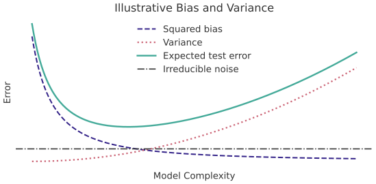
Fitting a quadratic can reduce bias when the true mean is curved. Higher-degree fits may follow noise in the sampled points, making predictions vary more between training sets. These trends depend on the data and fitting procedure.
Derivation
Add and subtract the two means inside the residual: \[ Y-\hat f_D(x) =\underbrace{Y-\mu(x)}_{\text{label variation}} +\underbrace{\mu(x)-\bar f(x)}_{\text{systematic error}} +\underbrace{\bar f(x)-\hat f_D(x)}_{\text{fitting variation}}. \] The first and last terms have mean zero. The middle term is fixed. The fresh label is independent of the training set, so the product of the first and last terms also has mean zero. Squaring and averaging therefore leaves just the three squared terms: \[ \begin{aligned} \mathbb E_{D,Y}[(Y-\hat f_D(x))^2\mid X=x] &=\mathbb E_Y[(Y-\mu(x))^2\mid X=x]\\ &\quad +(\mu(x)-\bar f(x))^2 +\mathbb E_D[(\bar f(x)-\hat f_D(x))^2]. \end{aligned} \]
Averaging over the feature distribution of \(X\) gives \(\mathbb E_D[R(\hat f_D)]\), the population error averaged over training sets. A training label helped determine \(\hat f_D\), so the independence step fails for training error. An independent test set estimates population error for one fitted model. To measure prediction variance, collect new training data and refit.
For a fixed numerical prediction \(c\in\mathbb R\), there is no variation across training sets: \(\bar f(x)=c\) and the variance term is zero. Let \(R_x(c)\) denote its expected squared error at input \(x\). Substituting into the decomposition gives \[ R_x(c)=\mathbb E[(Y-c)^2\mid X=x] =\operatorname{Var}(Y\mid X=x)+(\mu(x)-c)^2. \] Only the second term depends on \(c\), so the best prediction is \(f^*(x)=\mu(x)\). This optimum is over all prediction rules. A restricted model class \(\mathcal F\) may not contain \(f^*\). Its population error is \[ R(f^*)=\mathbb E_X[\operatorname{Var}(Y\mid X)]. \] Here \(\mathbb E_X\) averages the conditional label variance over the feature distribution. The remaining irreducible error comes from label variation at a fixed input. More training data cannot remove it. Recording an additional informative feature may reduce it.
Here \(Y\) is either \(-1\) or \(1\) at a fixed input \(x\).
Expected squared error is the label variance plus the squared distance from the prediction to the mean. Predicting the mean minimizes this error.
Outputs
Prediction Error
Choosing the Evaluation Data
Overfitting can occur even when training and test examples come from the same population. With distribution shift, the evaluation population differs from the population we want to predict. Let \(Q\) be the joint distribution of our test examples, while future examples follow \(P\). Write \(R_P(f)=R(f)\) to emphasize the target population, and let \(\widehat R_{\mathrm{test}}(f)\) be the empirical error on the test set. For a fixed \(f\) and independent test examples from \(Q\) with finite expected loss, increasing the test sample size gives \[ \widehat R_{\mathrm{test}}(f)\longrightarrow \mathbb E_{(X,Y)\sim Q}[(Y-f(X))^2]. \] This limit measures error under \(Q\), which can differ from the target risk \(R_P(f)\). For example, if the goal is to predict future observations, train on earlier data and test on later data. A random split of old observations would only measure performance on more examples from that earlier period.
Data leakage lets held-out information affect the fit or model choice. For example, estimate feature means and scales on the training set, then apply those same values to validation and test data. Calculating them from the full dataset would let held-out observations influence the fit.
Test error can rise near the point where training error first reaches zero, then fall as we add parameters. We will study this double descent in our class on generalization.