Principal Component Analysis
An image can have millions of pixels. A scientific experiment can record thousands of measurements for each observation. We can give all of these numbers to a learning algorithm, but many may contain similar information. Keeping fewer coordinates would make the data easier to store, compare, and use for prediction. With just two or three coordinates, we could even plot the observations and look for groups or outliers.
The challenge is deciding what to keep. In Low-Rank Approximation, we used the SVD to approximate a matrix using fewer directions. Principal component analysis (PCA) applies this idea to data: choose the directions along which the observations vary most, and represent each observation by its coordinates along those directions.
We’ll measure what we lose by how well we can reconstruct the original observations. This gives us an optimal linear representation, and a way to understand what happens when we compare examples in the smaller space.
Encoding and Reconstructing Data
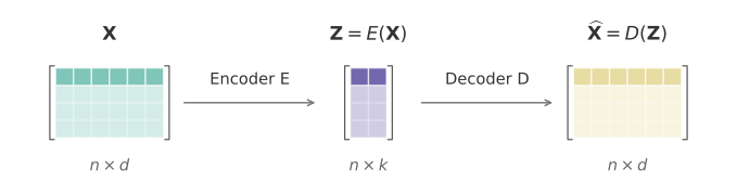
Put \(n\) examples with \(d\) features into a matrix \(\mathbf X\in\mathbb R^{n\times d}\), with example \(i\) in row \(\mathbf x_i^\top\). We’ll assume the columns are centered, i.e., we’ve already subtracted each feature’s mean. Zero then represents an average example. Centering matters because we want to describe how examples differ from the average, rather than spend a direction representing a shared offset.
We’d like to replace each row by just \(k\) numbers. An encoder \(E\) does the compression, and a decoder \(D\) tries to recover the original features. Applying them to each row gives us a matrix of embeddings \(\mathbf Z\) and a reconstruction \(\widehat{\mathbf X}\):
\[ \mathbf Z=E(\mathbf X)\in\mathbb R^{n\times k},\qquad \widehat{\mathbf X}=D(\mathbf Z)\in\mathbb R^{n\times d}. \]
Each row \(\mathbf z_i^\top\) of \(\mathbf Z\) is a \(k\)-dimensional embedding of one example. The reconstruction has the original \(d\) features, so we can compare it directly with the input. The embedding and reconstruction describe the same retained information in different coordinates.
PCA chooses these coordinates using the SVD. Let \(r\) be the rank of \(\mathbf X\) and choose \(1\leq k\leq r\) with \(k<d\). Collect its first \(k\) right singular vectors in \(\mathbf V_k\in\mathbb R^{d\times k}\). These are the principal directions, and they’re orthonormal: \(\mathbf V_k^\top\mathbf V_k=\mathbf I_k\). To encode and decode, we simply multiply:
\[ \mathbf Z=E(\mathbf X)=\mathbf X\mathbf V_k,\qquad \widehat{\mathbf X}=D(\mathbf Z)=\mathbf Z\mathbf V_k^\top. \]
The encoder takes an inner product with each principal direction. The decoder adds those directions back together, weighted by the resulting coordinates. It can put the example back in the span of the principal directions, but it can’t recover a component perpendicular to that span.
Below, we’re compressing three-dimensional points into two coordinates. On the left, the highlighted example \(\mathbf x_i\) projects onto the principal plane at \(\widehat{\mathbf x}_i\). On the right, \(\mathbf z_i\) records where it lands within that plane. The dashed segment shows what we lose. Drag the left view to see that segment from another angle; the embedding stays fixed because we’re only moving the camera.
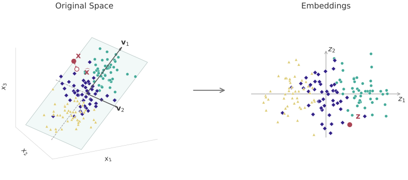
Once we’ve found the principal directions, we can use them to encode new examples too. Subtract the training feature means from the new example, then take its inner products with the same directions. After decoding, add those same means back to return to the original units. We don’t fit a new PCA basis for each example: all the embeddings need to use the same coordinates to be comparable.
Why PCA Is Optimal
We’ve described how to compress and reconstruct the data. To decide whether we chose good directions, we’ll use the squared Frobenius reconstruction error:
\[ \|\mathbf X-\widehat{\mathbf X}\|_F^2 =\sum_{i=1}^n\|\mathbf x_i-\widehat{\mathbf x}_i\|_2^2. \]
This adds up the squared error in every feature of every example. Keeping coordinates that help reconstruct many observations reduces this error; keeping a direction with almost no variation does little to help.
Write the rank-\(r\) SVD as \(\mathbf X=\mathbf U_r\boldsymbol\Sigma_r\mathbf V_r^\top\). Because the right singular vectors are orthonormal, multiplying by \(\mathbf V_k\) keeps exactly the first \(k\) terms. Decoding gives
\[ \mathbf Z=\mathbf X\mathbf V_k=\mathbf U_k\boldsymbol\Sigma_k,\qquad \widehat{\mathbf X}=\mathbf Z\mathbf V_k^\top=\mathbf U_k\boldsymbol\Sigma_k\mathbf V_k^\top=\mathbf X_k. \]
So PCA reconstructs the truncated SVD. The Eckart–Young–Mirsky theorem tells us that this minimizes Frobenius error among all matrices of rank at most \(k\):
\[ \|\mathbf X-\widehat{\mathbf X}\|_F^2 =\min_{\operatorname{rank}(\mathbf B)\leq k}\|\mathbf X-\mathbf B\|_F^2 =\sum_{j=k+1}^{r}\sigma_j^2. \]
Any linear encoder and linear decoder that pass through \(k\) coordinates produce a reconstructed matrix of rank at most \(k\). PCA attains the best error allowed by that rank constraint. No other pair of linear maps can reconstruct this data matrix with smaller squared error using the same number of coordinates. This is a statement about reconstruction on the data we used to fit PCA. It doesn’t say that these coordinates are best for every prediction task.
The singular values also help us decide how many coordinates to keep. Since \(\mathbf X\) is centered, \(\|\mathbf X\|_F^2=\sum_{j=1}^r\sigma_j^2\) measures the total squared variation around the mean. PCA retains \(\sum_{j=1}^k\sigma_j^2\) and discards the rest. The fraction retained is
\[ \frac{\sum_{j=1}^k\sigma_j^2}{\sum_{j=1}^r\sigma_j^2}. \]
This is often called the fraction of variance explained. Dividing each squared singular value by \(n-1\) gives the corresponding eigenvalue of the sample covariance matrix, so the common factor cancels in the fraction. A rapidly decreasing spectrum means that a few coordinates preserve most of the variation. A flat spectrum means that each discarded coordinate costs us a comparable amount.
The units of the features matter here. Changing one feature from meters to centimeters multiplies its squared contribution to the loss by \(100^2\). Centering removes a shared offset; it doesn’t remove differences in scale. We can scale features before fitting PCA if equal changes in their recorded units shouldn’t receive equal weight. That changes the reconstruction problem we’re asking PCA to solve.
In the demo, we’ll vary \(k\) and compare the measured reconstruction error with the discarded singular values. We’ll also check distances between individual observations. Optimal total reconstruction error doesn’t mean that every individual relationship survives compression.
What Happens to an Example and Its Distances?
Let’s look more closely at \(\mathbf x_i\), \(\widehat{\mathbf x}_i\), and \(\mathbf z_i\). The first two are vectors in the original \(d\)-dimensional feature space. The last has only \(k\) coordinates. To see exactly what they retain, extend the principal directions to a full orthonormal eigenbasis \(\mathbf v_1,\ldots,\mathbf v_d\) of \(\mathbf X^\top\mathbf X\), ordered by decreasing eigenvalue. These are the right singular vectors, including directions with eigenvalue zero if the data have rank less than \(d\).
Every example has an expansion in this basis:
\[ \mathbf x_i=\sum_{j=1}^{d}(\mathbf v_j^\top\mathbf x_i)\mathbf v_j. \]
PCA keeps the first \(k\) coefficients. For a column-vector example, encoding and decoding are
\[ \mathbf z_i=\mathbf V_k^\top\mathbf x_i,\qquad \widehat{\mathbf x}_i=\mathbf V_k\mathbf z_i=\sum_{j=1}^{k}(\mathbf v_j^\top\mathbf x_i)\mathbf v_j. \]
These are the same operations as before, transposed because examples occupy rows of \(\mathbf X\). For a training example, the \(j\)th embedding coordinate is \(\mathbf v_j^\top\mathbf x_i=\sigma_j U_{ij}\). Here \(U_{ij}\) is entry \((i,j)\) of \(\mathbf U_r\). The right singular vector \(\mathbf v_j\) tells us which combination of features we’re measuring; column \(j\) of \(\mathbf U_k\boldsymbol\Sigma_k\) lists that measurement across all examples.
The part we discarded uses only the remaining basis vectors:
\[ \mathbf r_i=\mathbf x_i-\widehat{\mathbf x}_i=\sum_{j=k+1}^{d}(\mathbf v_j^\top\mathbf x_i)\mathbf v_j. \]
The reconstruction and residual are perpendicular because every retained basis vector is perpendicular to every discarded one. The same is true when we take differences between examples: the reconstructed difference uses the first \(k\) basis vectors, and the residual difference uses the rest. This gives us an exact account of what happens to distance.
Claim: For two examples encoded with the same orthonormal PCA directions,
\[ \|\mathbf x_i-\mathbf x_j\|_2^2=\|\mathbf z_i-\mathbf z_j\|_2^2+\|\mathbf r_i-\mathbf r_j\|_2^2. \]
In particular, PCA never increases a Euclidean distance.
Proof
Split the difference into its retained and discarded parts:
\[ \mathbf x_i-\mathbf x_j=(\widehat{\mathbf x}_i-\widehat{\mathbf x}_j)+(\mathbf r_i-\mathbf r_j). \]
As we saw from their basis expansions, these two parts are perpendicular. The Pythagorean theorem therefore gives
\[ \|\mathbf x_i-\mathbf x_j\|_2^2=\|\widehat{\mathbf x}_i-\widehat{\mathbf x}_j\|_2^2+\|\mathbf r_i-\mathbf r_j\|_2^2. \]
Finally, \(\widehat{\mathbf x}_i-\widehat{\mathbf x}_j=\mathbf V_k(\mathbf z_i-\mathbf z_j)\). Multiplying by \(\mathbf V_k\) preserves lengths because its columns are orthonormal:
\[ \|\mathbf V_k(\mathbf z_i-\mathbf z_j)\|_2^2=(\mathbf z_i-\mathbf z_j)^\top\mathbf V_k^\top\mathbf V_k(\mathbf z_i-\mathbf z_j)=\|\mathbf z_i-\mathbf z_j\|_2^2. \]
Substituting gives the claimed identity. The discarded squared distance is nonnegative, so the embedding distance cannot exceed the original distance.
PCA preserves a pair’s distance exactly when the two examples have the same discarded part. At the other extreme, two examples that differ only in discarded directions get identical embeddings. Different pairs can lose different amounts of distance, so the nearest neighbor can change even though PCA minimizes total reconstruction error. A feature that barely varies may also be essential for predicting a label: reconstruction error alone doesn’t tell us which differences matter for that task.
We now have a way to compress numerical data and understand what the compression loses. In Embeddings, we’ll apply it to words, then ask what we can gain from nonlinear maps and from training objectives that directly reward similarity.