Embeddings

In Principal Component Analysis, we learned to represent numerical data with fewer coordinates. But for text, we first have to decide which numbers to use. We could number the words in a dictionary, but nearby numbers would tell us about alphabetical order. We’d rather have cat close to dog because they mean similar things. Before a neural network can do anything with text, we need a vector representation.

These representations are called embeddings. PCA gives us one way to make them, once we’ve turned the words into numerical features. Neural networks let us learn more flexible representations, and changing the training objective lets us choose which relationships they preserve.

How should we turn our data into vectors?

We’ll start by applying PCA to word counts, then use nonlinear encoders to preserve more complicated structure and contrastive learning to reward similarity directly.

Word Embeddings from Co-occurrence

Now let’s try this with words. One simple representation gives every word its own coordinate: put a one there and zeros everywhere else. This is a one-hot vector. It tells us which word we have, but every pair of distinct words is the same distance apart. We’d still have no reason to put cat closer to dog than to truck.

We can learn something about a word from the company it keeps. For each occurrence of dog, count the words nearby, e.g., the two words on either side within the sentence. Repeat for every word to build a co-occurrence matrix. Each row is a word, each column is a context word, and each entry counts how often they appear together in the window.

Here’s a small example with made-up counts:

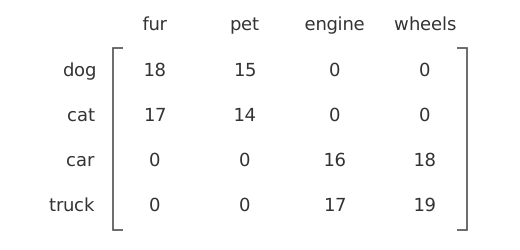
Dog and cat appear near the same words, so their rows are similar. The same is true of car and truck. We now have numerical features that say something about how words are used, but with a large vocabulary, each row could have thousands of entries.

This is where PCA helps. Subtract each column’s mean to get \(\mathbf X\), then use our encoder to compute \(\mathbf Z=E(\mathbf X)\). Each row is now a short word embedding. The decoder tries to recover the centered counts from those few coordinates, just as it reconstructed the numerical features in the PCA reading.

In the demo, we’ll change the number of coordinates and check both the reconstructed counts and which words end up close together.

The counts we choose matter. Very frequent words can dominate squared error, so we might first replace each count by \(\log(1+\text{count})\) and then center. Large counts become less dominant, changing which differences PCA tries hardest to preserve.

Word embeddings can also capture relationships as directions. The change from dog to puppy gives us a direction we can add to cat. Likewise, we can try adding the change from man to woman to wizard.

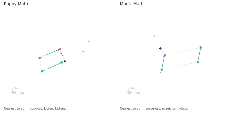
These plots use GloVe word vectors, learned from co-occurrence counts. Each shows a three-dimensional PCA view of the words and nearby tokens. The arrows copy the same change from one word to another. Nearby tokens are chosen by cosine similarity in the original embedding space, so rotating the view doesn’t change the matches. The arithmetic is approximate: look at which words end up nearest the sum.

There’s also a limitation we can’t fix by keeping more coordinates: bank has just one row. The counts mix together river bank and bank loan, so both uses get the same embedding. Later, we’ll see how language models give a word different representations depending on its sentence.

Nonlinear Autoencoders

Eckart–Young–Mirsky tells us we’ve found the best linear reconstruction. But why stop at linear maps? If the data lie along a curve, we may only need one number to say where we are on it. A nonlinear decoder can turn that number back into a point on the curve.

A manifold is a nonlinear analogue of a subspace. We can use fewer coordinates to identify where a point lies on it, but following its shape may require a nonlinear representation. For the rolled sheet below, each point has three coordinates, but we only need two to locate it on the sheet: how far along it lies and its height.

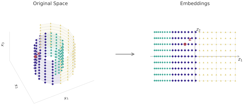
The colors and point shapes match across the two views, and the highlighted point shows the same example in each. The embedding unfolds the sheet. Projecting it onto a plane can put different layers on top of each other, while unfolding keeps those layers separate. Here we use the known surface coordinates to show the geometry. For real data, we need to learn an encoder and decoder that can follow the shape.

An autoencoder uses neural networks for \(E\) and \(D\) and trains them together to minimize

\[ \min_{E,D}\ \|\mathbf X-D(E(\mathbf X))\|_F^2. \]

Each network can have several layers with nonlinear activations. The variables we’re optimizing are the weights of the two networks. We feed an example through \(E\) and then \(D\), compare the reconstruction with the input, and backpropagate through both networks. Once trained, we can run a new input through \(E\) to get its embedding. Gradient descent may not find the best weights, but nonlinear maps give us reconstructions that PCA cannot produce.

But a better reconstruction isn’t always a better representation for our task. Suppose we want to recognize an animal in a photograph. Most pixels might belong to the background, so the autoencoder could reduce its error by preserving the grass while losing a small feature that identifies the animal. To get the embeddings we want, we may need to change what we reward.

Contrastive Learning

Suppose we have two photographs of the same animal, or two sentences that mean the same thing. We’d like their embeddings to be similar. Contrastive learning trains an encoder to find the matching example among other candidates. The match forms a positive pair, and we treat the other candidates as negative pairs.

Our encoder \(E\) can be a nonlinear neural network, just as in the autoencoder. This time, we train it to recognize matches. We don’t need a decoder or a reconstruction of the input.

Arrange \(n\geq2\) positive pairs in two batches \(\mathbf X\) and \(\mathbf X'\), so example \(i\) in one matches example \(i\) in the other. The prime marks the second batch. Apply the same encoder to each example and normalize its output to length one. Assuming the outputs are nonzero and including normalization in \(E\), we get

\[ \mathbf Z=E(\mathbf X),\qquad \mathbf Z'=E(\mathbf X'),\qquad \mathbf S=\mathbf Z(\mathbf Z')^\top. \]

Both embedding matrices have \(n\) rows and \(k\) columns. The \(n\times n\) matrix \(\mathbf S\) compares every embedding in the first batch with every embedding in the second. Its entry \(S_{ij}=\mathbf z_i^\top\mathbf z'_j\) is their cosine similarity, since the vectors have length one. The matrix multiplication computes these comparisons after the neural network has produced the embeddings.

Now look at row \(i\) of \(\mathbf S\). We have \(n\) scores, one for each candidate, and candidate \(i\) is the correct match. This is a classification problem! We can use the same softmax and cross-entropy we used in Logistic Regression.

First, turn the scores into probabilities. Write \(p_{ij}\) for the probability assigned to candidate \(j\) when finding a match for example \(i\):

\[ p_{ij}=\frac{\exp(S_{ij}/\tau)}{\sum_{k=1}^n\exp(S_{ik}/\tau)}. \]

The numerator increases with candidate \(j\)’s similarity. The denominator adds up all the candidates’ contributions, so each row of probabilities sums to one. The temperature \(\tau>0\) controls how strongly score differences affect these probabilities. A smaller temperature makes the distribution more concentrated on the highest scores. A larger temperature makes it more uniform.

The correct candidate is \(i\), so its probability is \(p_{ii}\). Cross-entropy takes the negative log of that probability, then we average over the batch:

\[ \ell_i=-\log p_{ii},\qquad \mathcal L=\frac1n\sum_{i=1}^n\ell_i. \]

To reduce the loss, the encoder must make the correct match stand out among the candidates. This is the contrastive cross-entropy objective used in methods such as SimCSE.

Let’s interpret what the gradient does. Substituting the softmax probability gives

\[ \ell_i=-\log p_{ii}=-\frac{S_{ii}}{\tau}+\log\left(\sum_{k=1}^n\exp(S_{ik}/\tau)\right). \]

Differentiating with respect to the matching score \(S_{ii}\) and a competing score \(S_{ij}\) gives

\[ \frac{\partial\ell_i}{\partial S_{ii}}=\frac{p_{ii}-1}{\tau}<0,\qquad \frac{\partial\ell_i}{\partial S_{ij}}=\frac{p_{ij}}{\tau}>0\quad(j\ne i). \]

Gradient descent therefore favors increasing the matching score and decreasing competing scores, with larger corrections for competitors assigned high probability. Backpropagation carries these gradients through the embeddings to update \(E\).

Why include the other candidates? If we only rewarded similarity within positive pairs, \(E\) could give every input the same unit vector. This is called collapse. Here, all the scores would be equal, giving \(p_{ij}=1/n\) and a loss of \(\log n\). The encoder would be no better at finding a match than a uniform guess.

The pairs still matter. Two sentences we treat as negatives may mean the same thing. The loss would then ask the encoder to distinguish examples we’d prefer to keep together. Choosing the pairs is part of choosing what our embeddings should preserve.

How Language Models Learn Embeddings

So which of these methods do large language models use? For a GPT-style model, the main training task is the one we discussed in TL;DR: predict the next token. The embeddings are learned along with the rest of the model, without first building a co-occurrence matrix or running PCA.

First, split the text into tokens: words, parts of words, or punctuation. Each token gets an initial vector from a learned table. Transformer layers then combine it with information from the preceding tokens to predict what comes next. Cross-entropy rewards the token that actually appeared in the text, and backpropagation updates both the initial vectors and the transformer weights. GPT-2 is an example.

This gives us a way to distinguish the two uses of bank. The initial table supplies the same vector for that token, but the transformer layers can change its representation using the surrounding text available to them. These are contextual embeddings. What they learn to keep is shaped by the prediction task: information that helps predict the next token reduces the training loss.

Another option is to hide some tokens and ask the model to recover them. BERT trains this way, using text on both sides of a masked token. This resembles a denoising autoencoder: we damage the input and ask the model to recover the missing information. Here, though, we’re predicting token identities with cross-entropy, rather than reconstructing numerical features with squared error.

Finally, suppose we want to search for sentences with similar meanings. Good next-token predictions don’t guarantee good sentence similarities. We can start with a pretrained language model and train it further on matching and nonmatching sentences, as in SimCSE. Contrastive training then rewards the relationships we want to use for search.

The same model can therefore learn from more than one objective: token prediction first, followed by contrastive training for sentence embeddings. In the Transformer reading, we’ll see how attention lets the model build representations using the other tokens in the text.