Gradient Descent in Practice
MNIST has 60,000 training images and 10,000 test images, each with \(28\times28\) pixels. To train a neural network with full gradient descent, we run a forward and backward pass over all 60,000 training images before making even one update. Then we repeat that work for the next update.
Memory matters too. The training pixels alone occupy about 188 MB as 32-bit floating-point numbers, which fits comfortably in RAM. But training also stores intermediate activations for the backward pass. With larger images, datasets, and networks, processing everything at once can exceed the available RAM or GPU memory. We can compute a full gradient in smaller chunks to save memory, but we still have to process every training example before updating the weights.
A minibatch lets us update after just a small group of examples, keeping only that batch’s activations in memory.
We will estimate the full gradient from a batch, measure the sampling error, and use recent gradients to choose the direction and scale of each update.
Minibatch Gradients
For \(n\) training examples, let \(\ell_i\) be the loss of example \(i\) at the current \(P\) weights \(\mathbf w\in\mathbb R^P\). All gradients are with respect to these weights, and we leave \(\mathbf w\) out of the notation when it is clear from context. The loss and its gradient are averages: \[ \mathcal L=\frac1n\sum_{i=1}^n\ell_i, \qquad \nabla\mathcal L=\frac1n\sum_{i=1}^n\nabla\ell_i. \]
Draw \(B\) example indices \(i_1,\ldots,i_B\) independently and uniformly from \(\{1,\ldots,n\}\). An example can appear more than once. Call this minibatch \(S\), and average its losses: \[ \ell_S=\frac1B\sum_{b=1}^B\ell_{i_b}, \qquad \nabla\ell_S=\frac1B\sum_{b=1}^B\nabla\ell_{i_b}. \] Computing this gradient uses only \(B\) examples instead of \(n\). For MNIST, a batch of \(128\) lets us update after processing \(128\) images rather than waiting for all \(60{,}000\).
Claim: At fixed weights, the minibatch gradient is unbiased: \[ \mathbb E_S[\nabla\ell_S]=\nabla\mathcal L. \]
Proof
For any draw \(b=1,\ldots,B\), each example has probability \(1/n\), so \[ \mathbb E[\nabla\ell_{i_b}] =\sum_{i=1}^n\Pr(i_b=i)\nabla\ell_i =\frac1n\sum_{i=1}^n\nabla\ell_i =\nabla\mathcal L. \] Averaging over the \(B\) draws gives \[ \mathbb E_S[\nabla\ell_S] =\frac1B\sum_{b=1}^B\mathbb E[\nabla\ell_{i_b}] =\nabla\mathcal L. \]
We compute each example’s gradient with the same forward and backward passes as in Neural Networks. The forward pass ends at the loss \(\ell\), and the backward pass gives its derivatives.


Stochastic gradient descent (SGD) updates the weights using the minibatch gradient: \[ \mathbf w^{(t+1)}=\mathbf w^{(t)}-\alpha\nabla\ell_{S^{(t)}}. \] Here \(\alpha>0\) is the learning rate and \(S^{(t)}\) is the batch at step \(t\). Each update costs \(O(BP)\) for a dense network with \(P\) parameters. We can take many updates before doing as much work as one full gradient.
One epoch is one dataset’s worth of training examples. In practice, we often shuffle the dataset and visit every example once per epoch. The claims here use independent draws with replacement, which makes the sampling error especially simple to analyze.
Gradient Variance
An unbiased gradient can still point away from the full gradient on a particular step. To measure this disagreement, define \[ \sigma^2=\frac1n\sum_{i=1}^n\|\nabla\ell_i-\nabla\mathcal L\|_2^2. \] This is the expected squared error from using one randomly chosen example.
Claim: At fixed weights, a batch of \(B\) independent uniform draws has expected squared gradient error \[ \mathbb E_S\!\left[\|\nabla\ell_S-\nabla\mathcal L\|_2^2\right] =\frac{\sigma^2}{B}. \]
Proof
For draw \(b=1,\ldots,B\), let \(\mathbf e_b=\nabla\ell_{i_b}-\nabla\mathcal L\in\mathbb R^P\) be its gradient error. These independent vectors have mean zero by the previous claim, and \(\mathbb E\|\mathbf e_b\|_2^2=\sigma^2\) by definition. When we expand the squared length of their sum, each cross term has expectation zero: for \(b\ne c\), \[ \mathbb E[\mathbf e_b^\top\mathbf e_c] =(\mathbb E[\mathbf e_b])^\top\mathbb E[\mathbf e_c]=0. \] This is the same mechanism as the variance of an independent sum, now for vector errors. Only the \(B\) squared lengths remain, giving \[ \begin{aligned} \mathbb E\!\left[\|\nabla\ell_S-\nabla\mathcal L\|_2^2\right] &=\frac1{B^2}\mathbb E\!\left[\left\|\sum_{b=1}^B\mathbf e_b\right\|_2^2\right]\\ &=\frac1{B^2}\sum_{b=1}^B\mathbb E\|\mathbf e_b\|_2^2 =\frac{\sigma^2}{B}. \end{aligned} \]
The root mean squared error is \(\sigma/\sqrt B\). Halving it requires four times as many examples. A larger batch gives a steadier direction, but each update costs more.
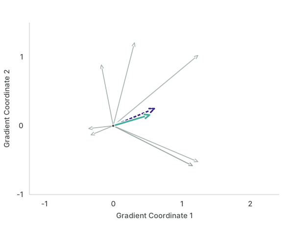
Near a minimum, individual examples can still have nonzero gradients even when their average is zero. Reducing the learning rate or increasing the batch size makes these late updates steadier.
Momentum
A small batch makes an update affordable, but even using the full gradient can be inefficient. Next, we’ll discuss two ways of using information from prior gradient updates. There are two complementary uses of this history: momentum combines recent directions, and adaptivity adjusts the scale for each weight. Adam will use both.
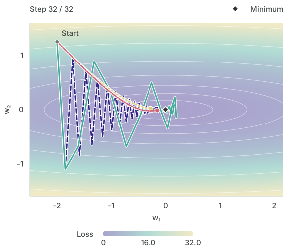
Suppose a gradient coordinate keeps the same sign across several batches. Those batches agree on which way to move that weight. If the sign keeps changing, their contributions can partly cancel.
Momentum keeps some of the previous step’s direction: \[ \mathbf v^{(t+1)}=\beta\mathbf v^{(t)}+\nabla\ell_{S^{(t)}}, \qquad \mathbf w^{(t+1)}=\mathbf w^{(t)}-\alpha\mathbf v^{(t+1)}. \] Start with \(\mathbf v^{(0)}=\mathbf0\). The momentum factor \(0\leq\beta<1\) controls how much history remains. At \(\beta=0\), this is ordinary SGD. Larger \(\beta\) preserves more of the previous velocity, so there is less damping.
Components that repeatedly point the same way accumulate. Components that alternate tend to cancel. This can speed progress along a valley, though too much momentum can carry the weights past the minimum.
This also helps on the elongated loss surfaces from Gradient Descent: gradients can alternate across the steep direction while agreeing along the shallow direction.
Adaptive Step Sizes
We also need to choose how far to move each weight. One gradient coordinate might regularly be much larger than another because the corresponding features have different scales. Momentum can preserve useful directions while leaving this mismatch in scale.
Adaptivity uses recent gradient magnitudes to choose a multiplier for each coordinate. Write \(\partial_j\ell=\partial\ell/\partial w_j\) for the derivative with respect to weight \(j\). For each weight \(j=1,\ldots,P\), keep a running average \(s_j\) of squared gradients, starting at \(s_j=0\). When a new minibatch \(S\) arrives, update it: \[ s_j\leftarrow\gamma s_j+(1-\gamma)(\partial_j\ell_S)^2. \] Here \(0\leq\gamma<1\) controls how much history we keep. Squaring measures magnitude, so positive and negative gradients do not cancel.
After \(t\geq1\) updates, take a square root to return to the scale of the gradients: \[ r_j=\sqrt{\frac{s_j}{1-\gamma^t}}+\epsilon. \] Dividing by \(1-\gamma^t\) corrects for starting the average at zero. The small constant \(\epsilon>0\) prevents division by zero. Now use this scale in the weight update: \[ w_j\leftarrow w_j-\frac{\alpha}{r_j}\,\partial_j\ell_S. \] The base learning rate is \(\alpha\), and coordinate \(j\) uses the effective learning rate \(\alpha/r_j\). A coordinate with larger recent gradients gets a smaller multiplier. This is the scaling used by RMSProp, with the correction for starting at zero.
Adam combines the two ideas in one update. Let \(\widehat m_j\) be an exponentially weighted average of recent gradients in coordinate \(j\), normalized so its weights sum to one. Adam divides this average by the adaptive scale: \[ w_j\leftarrow w_j-\alpha\frac{\widehat m_j}{r_j}. \] The numerator averages signed gradients, so opposing directions can cancel. The denominator averages squared gradients, so both signs contribute to the scale. A coordinate whose gradients keep reversing can therefore have a small numerator even when its gradient magnitudes are large. The two averages can use different amounts of history. The Adam documentation gives the full update.
We can now train on a small batch, take an update that uses recent gradient information, and move on to the next batch. In the demo, we train a neural network on MNIST with PyTorch, cross-entropy loss, and Adam.