Embeddings

So far, we’ve assumed that our data arrive as vectors of numbers. For an image, we can simply list the pixel values. But that gives us millions of coordinates, many of which contain similar information. We’d like to use fewer numbers so our algorithms run faster, while keeping the features we need to make predictions.

For text, we first have to decide which numbers to use. We could number the words in a dictionary, but nearby numbers would tell us about alphabetical order. We’d rather have cat close to dog because they mean similar things. Before a neural network can do anything with text, we need to choose a vector representation.

These representations are called embeddings. We’ll begin with PCA, which uses the SVD to reduce the dimension of numerical data, and then apply it to words. Next, we’ll use neural networks to learn nonlinear embeddings and see how changing the training objective changes what they preserve.

How should we turn our data into vectors?

Principal Component Analysis

Let \(\mathbf X\in\mathbb R^{n\times d}\) contain \(n\) examples with \(d\) features, with example \(i\) in row \(\mathbf x_i^\top\). Assume its columns are already centered: we have subtracted each feature’s mean. Centering makes zero represent an average example.

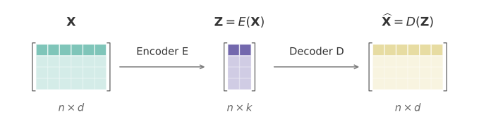
We want an encoder \(E\) that gives each example \(1\leq k<d\) coordinates and a decoder \(D\) that reconstructs the original features. We apply these maps to each row of a matrix:

\[ \begin{aligned} \mathbf Z&=E(\mathbf X)\in\mathbb R^{n\times k},\\[.4em] \widehat{\mathbf X}&=D(\mathbf Z)\in\mathbb R^{n\times d}. \end{aligned} \]

Each row \(\mathbf z_i^\top\) of \(\mathbf Z\) is an embedding. We will keep \(E\), \(D\), and \(\mathbf Z\) for these same roles throughout the reading.

Principal component analysis (PCA) chooses the embedding coordinates using the SVD of the centered data. Take \(k\) no larger than the rank of \(\mathbf X\), and put its first \(k\) right singular vectors into \(\mathbf V_k\in\mathbb R^{d\times k}\). These orthonormal columns are the principal directions. PCA uses

\[ \begin{aligned} \mathbf Z=E(\mathbf X)&=\mathbf X\mathbf V_k,\\[.4em] D(\mathbf Z)&=\mathbf Z\mathbf V_k^\top. \end{aligned} \]

The encoder takes inner products with the principal directions. The decoder uses those coordinates to combine the same directions. Thus the reconstruction is the projection onto their span.

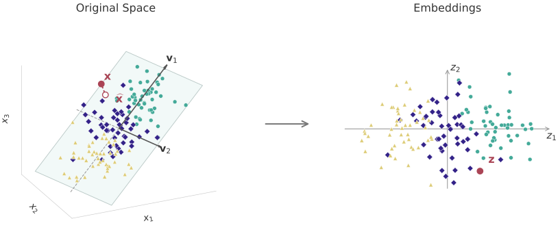
In the figure below, each three-dimensional point gets a two-dimensional embedding. The highlighted point projects onto the plane, and its embedding gives the two coordinates of that projection. The dashed segment is the part the decoder cannot recover.

We measure reconstruction error with the squared Frobenius norm. It adds the squared errors over all features of all examples:

\[ \|\mathbf X-\widehat{\mathbf X}\|_F^2 =\sum_{i=1}^n\|\mathbf x_i-\widehat{\mathbf x}_i\|_2^2. \]

Projection keeps the first \(k\) right singular directions and removes the rest. This gives exactly the rank-\(k\) truncated SVD reconstruction \(\mathbf X_k\):

\[ D(E(\mathbf X))=\mathbf X\mathbf V_k\mathbf V_k^\top=\mathbf X_k. \]

The Eckart–Young–Mirsky theorem already tells us that this minimizes Frobenius error among matrices of rank at most \(k\). Any linear encoder and decoder with \(k\) embedding coordinates produce a reconstruction of rank at most \(k\). So PCA achieves the best reconstruction error available to those linear maps.

For a new example, subtract the training feature means before encoding. Add those means back after decoding to return to the original units. PCA is useful for compression and for plotting high-dimensional data in two or three dimensions. It preserves directions with large variation, which need not be the directions most useful for a prediction task.

Word Embeddings from Co-occurrence

To apply PCA to words, we first need a numerical description of each word. A one-hot vector puts a one in the coordinate for that word and zeros elsewhere. This identifies the word, but every pair of distinct one-hot vectors has the same distance. The representation gives us no reason to put cat closer to dog than to truck.

Instead, count the words that appear nearby. Choose a window, such as the two words on either side within a sentence. Make a co-occurrence matrix with one row per word and one column per context word. Each entry counts how often that context appears in the chosen window around the row’s word.

For example, a few rows and columns might look like this:

Word / context	fur	pet	engine	wheels
dog	18	15	0	0
cat	17	14	0	0
car	0	0	16	18
truck	0	0	17	19

These illustrative counts give dog and cat similar context profiles. Car and truck share a different profile. With a large vocabulary, each row could have thousands of context coordinates.

Subtract each column’s mean to obtain the centered matrix \(\mathbf X\), then apply the PCA encoder \(E\) from the previous section. Each row of \(\mathbf Z=E(\mathbf X)\) is now a short word embedding. Its decoder reconstructs that word’s centered context profile. The leading directions summarize patterns shared across context words, so we can compare words without keeping every count.

The demo lets us change the embedding dimension and compare reconstructed context profiles.

Raw counts give frequent words considerable influence. We can also apply PCA after rescaling the counts, for example by taking \(\log(1+\text{count})\) before centering. This changes which differences the reconstruction loss emphasizes.

The table has just one row for bank, so it merges the uses in river bank and bank loan. We will return to representations that depend on the surrounding sentence in the final section.

Nonlinear Autoencoders

PCA solves the linear reconstruction problem. If the data follow a curved shape, we may be able to reconstruct them more accurately with nonlinear maps.

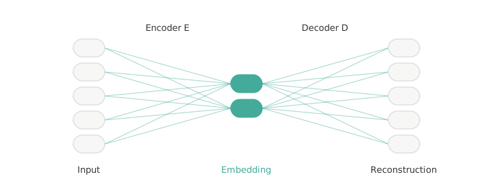
An autoencoder learns an encoder \(E\) and decoder \(D\) together. Replace the PCA maps by neural networks, keeping the same \(k\)-dimensional embeddings and the same reconstruction objective:

\[ \min_{E,D}\ \|\mathbf X-D(E(\mathbf X))\|_F^2. \]

Here we optimize the weights of the two networks. Backpropagation carries reconstruction errors through \(D\) and then through \(E\), so both networks learn from the same loss. Once trained, \(E\) can produce an embedding for a new input in one forward pass.

For example, points along a parabola can be described by one coordinate. A nonlinear decoder can turn that coordinate into a point on the curve. A linear decoder with one embedding coordinate can only produce points on a line.

This does not contradict Eckart–Young–Mirsky. The matrix reconstructed by a nonlinear decoder need not have rank at most \(k\). We have changed the set of reconstructions we can produce. The SVD no longer solves the optimization problem, and gradient descent is not guaranteed to find the best network weights.

A small embedding can force the network to share information across features, but reconstruction alone does not tell it which features we care about. For an animal photograph, accurately reconstructing the background may reduce squared error more than preserving a small feature that distinguishes the animal. We can choose an objective that directly rewards useful similarities instead.

Contrastive Learning

Contrastive learning uses pairs of related examples to train an encoder. A positive pair might be two views of the same photograph or two sentences expressing the same idea. Other examples in the batch serve as negative pairs: the encoder should distinguish them from the match.

Arrange \(n\geq2\) positive pairs in two batches \(\mathbf X\) and \(\mathbf X'\), with matching examples in the same row. The prime simply marks the second batch. This objective does not require PCA centering. Apply the same encoder to both and normalize each nonzero output to length one:

\[ \begin{aligned} \mathbf Z&=E(\mathbf X),\qquad \mathbf Z'=E(\mathbf X'),\\[.4em] \mathbf S&=\mathbf Z(\mathbf Z')^\top. \end{aligned} \]

Here \(E\) includes the normalization step. Both embedding matrices have \(n\) rows and \(k\) columns. The entry \(S_{ij}\) is the dot product between embedding \(i\) in the first batch and embedding \(j\) in the second. Since the vectors have unit length, this is their cosine similarity.

The diagonal of \(\mathbf S\) compares matched pairs. Off-diagonal entries compare mismatched pairs. A simple similarity-matching loss is

\[ \mathcal L=\|\mathbf S-\mathbf I_n\|_F^2, \]

where \(\mathbf I_n\) is the \(n\times n\) identity matrix. This asks matched pairs to have similarity one and mismatched pairs to have similarity zero. For unit vectors, similarity one means the vectors are identical, and similarity zero means they are perpendicular. We have reused squared error, now to fit a matrix of desired similarities instead of reconstructing inputs.

Both parts matter. If we rewarded only matched pairs, the encoder could give every input the same unit vector. Every positive pair would match perfectly, but the embeddings would contain no information. With the full matrix loss, that constant encoder also gives every mismatched pair similarity one, so the off-diagonal entries incur error. This is how the negative pairs discourage collapse.

The identity is a target, not a guarantee of zero loss. If \(n>k\), then \(\mathbf S\) has rank at most \(k\) and cannot equal the rank-\(n\) identity. Also, two examples chosen as negatives may actually be related. The choice of pairs and embedding dimension affects what the encoder can learn.

This squared-error objective is a simple way to study contrastive learning. Widely used methods also turn similarities into probabilities and use cross-entropy. The shared idea is to reward matches while distinguishing them from other candidates.

How Language Models Learn Embeddings

A GPT-style language model learns its representations by predicting the next token. It does not need a precomputed co-occurrence matrix or a PCA step. Text is split into tokens, which can be words, parts of words, or punctuation. A learned table supplies an initial vector for each token, and transformer layers combine that vector with information from preceding tokens. The model predicts the next token from the resulting representation. Training uses cross-entropy on the observed next token, and backpropagation updates both the embedding table and the transformer weights. GPT-2 is an example of this training setup.

The initial table gives a token the same vector wherever it appears. The layers above it produce contextual embeddings: the representation of bank can differ between river bank and bank loan. These internal representations serve token prediction. They need not have the same geometry as embeddings trained for similarity search.

Language models can also learn from missing tokens. BERT masks some input tokens and learns to predict them using the surrounding text. This resembles a denoising autoencoder, but its targets are token identities and its loss is cross-entropy, rather than the numerical squared reconstruction error above.

For sentence search, we often want one vector per sentence whose similarity reflects meaning. A pretrained language model can be further trained with a contrastive objective for that purpose, as in SimCSE. Thus token prediction and contrastive learning can be successive stages, with different objectives shaping the representations.

A useful embedding keeps the distinctions needed by its training task. The Transformer reading will show how attention builds contextual representations for token prediction.